8. The OpenMM Library: Introduction
8.1. What Is the OpenMM Library?
OpenMM consists of two parts. First, there is a set of libraries for performing many types of computations needed for molecular simulations: force evaluation, numerical integration, energy minimization, etc. These libraries provide an interface targeted at developers of simulation software, allowing them to easily add simulation features to their programs.
Second, there is an “application layer”, a set of Python libraries providing a high level interface for running simulations. This layer is targeted at computational biologists or other people who want to run simulations, and who may or may not be programmers.
The first part of this guide focused on the application layer and described how to run simulations with it. We now turn to the lower level libraries. We will assume you are a programmer, that you are writing your own applications, and that you want to add simulation features to those applications. The following chapters describe how to do that with OpenMM.
8.1.1. How to get started
We have provided a number of files that make it easy to get started with OpenMM. Pre-compiled binaries are provided for quickly getting OpenMM onto your computer (See Chapter 3 for set-up instructions). We recommend that you then compile and run some of the tutorial examples, described in Chapter 10. These highlight key functions within OpenMM and teach you the basic programming concepts for using OpenMM. Once you are ready to begin integrating OpenMM into a specific software package, read through Chapter 13 to see how other software developers have done this.
8.1.2. License
Two different licenses are used for different parts of OpenMM. The public API, the low level API, the reference platform, the CPU platform, and the application layer are all distributed under the MIT license. This is a very permissive license which allows them to be used in almost any way, requiring only that you retain the copyright notice and disclaimer when distributing them.
The CUDA and OpenCL platforms are distributed under the GNU Lesser General Public License (LGPL). This also allows you to use, modify, and distribute them in any way you want, but it requires you to also distribute the source code for your modifications. This restriction applies only to modifications to OpenMM itself; you need not distribute the source code to applications that use it.
OpenMM also uses several pieces of code that were written by other people and are covered by other licenses. All of these licenses are similar in their terms to the MIT license, and do not significantly restrict how OpenMM can be used.
All of these licenses may be found in the “licenses” directory included with OpenMM.
8.2. Design Principles
The design of the OpenMM API is guided by the following principles.
- The API must support efficient implementations on a variety of architectures.
The most important consequence of this goal is that the API cannot provide direct access to state information (particle positions, velocities, etc.) at all times. On some architectures, accessing this information is expensive. With a GPU, for example, it will be stored in video memory, and must be transferred to main memory before outside code can access it. On a distributed architecture, it might not even be present on the local computer. OpenMM therefore only allows state information to be accessed in bulk, with the understanding that doing so may be a slow operation.
- The API should be easy to understand and easy to use.
This seems obvious, but it is worth stating as an explicit goal. We are creating OpenMM with the hope that many other people will use it. To achieve that goal, it should be possible for someone to learn it without an enormous amount of effort. An equally important aspect of being “easy to use” is being easy to use correctly. A well designed API should minimize the opportunities for a programmer to make mistakes. For both of these reasons, clarity and simplicity are essential.
- It should be modular and extensible.
We cannot hope to provide every feature any user will ever want. For that reason, it is important that OpenMM be easy to extend. If a user wants to add a new molecular force field, a new thermostat algorithm, or a new hardware platform, the API should make that easy to do.
- The API should be hardware independent.
Computer architectures are changing rapidly, and it is impossible to predict what hardware platforms might be important to support in the future. One of the goals of OpenMM is to separate the API from the hardware. The developers of a simulation application should be able to write their code once, and have it automatically take advantage of any architecture that OpenMM supports, even architectures that do not yet exist when they write it.
8.3. Choice of Language
Molecular modeling and simulation tools are written in a variety of languages: C, C++, Fortran, Python, TCL, etc. It is important that any of these tools be able to use OpenMM. There are two possible approaches to achieving this goal.
One option is to provide a separate version of the API for each language. These could be created by hand, or generated automatically with a wrapper generator such as SWIG. This would require the API to use only “lowest common denominator” features that can be reasonably supported in all languages. For example, an object oriented API would not be an option, since it could not be cleanly expressed in C or Fortran.
The other option is to provide a single version of the API written in a single language. This would permit a cleaner, simpler API, but also restrict the languages it could be directly called from. For example, a C++ API could not be invoked directly from Fortran or Python.
We have chosen to use a hybrid of these two approaches. OpenMM is based on an object oriented C++ API. This is the primary way to invoke OpenMM, and is the only API that fully exposes all features of the library. We believe this will ultimately produce the best, easiest to use API and create the least work for developers who use it. It does require that any code which directly invokes this API must itself be written in C++, but this should not be a significant burden. Regardless of what language we had chosen, developers would need to write a thin layer for translating between their own application’s data model and OpenMM. That layer is the only part which needs to be written in C++.
In addition, we have created wrapper APIs that allow OpenMM to be invoked from other languages. The current release includes wrappers for C, Fortran, and Python. These wrappers support as many features as reasonably possible given the constraints of the particular languages, but some features cannot be fully supported. In particular, writing plug-ins to extend the OpenMM API can only be done in C++.
We are also aware that some features of C++ can easily lead to compatibility and portability problems, and we have tried to avoid those features. In particular, we make minimal use of templates and avoid multiple inheritance altogether. Our goal is to support OpenMM on all major compilers and operating systems.
8.4. Architectural Overview
OpenMM is based on a layered architecture, as shown in the following diagram:
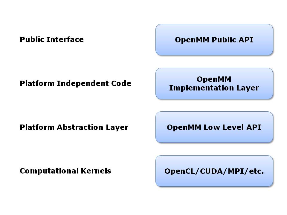
Figure 8-1: OpenMM architecture
At the highest level is the OpenMM public API. This is the API developers program against when using OpenMM within their own applications. It is designed to be simple, easy to understand, and completely platform independent. This is the only layer that many users will ever need to look at.
The public API is implemented by a layer of platform independent code. It serves as the interface to the lower level, platform specific code. Most users will never need to look at it.
The next level down is the OpenMM Low Level API (OLLA). This acts as an abstraction layer to hide the details of each hardware platform. It consists of a set of C++ interfaces that each platform must implement. Users who want to extend OpenMM will need to write classes at the OLLA level. Note the different roles played by the public API and the low level API: the public API defines an interface for users to invoke in their own code, while OLLA defines an interface that users must implement, and that is invoked by the OpenMM implementation layer.
At the lowest level is hardware specific code that actually performs computations. This code may be written in any language and use any technologies that are appropriate. For example, code for GPUs will be written in stream processing languages such as OpenCL or CUDA, code written to run on clusters will use MPI or other distributed computing tools, code written for multicore processors will use threading tools such as Pthreads or OpenMP, etc. OpenMM sets no restrictions on how these computational kernels are written. As long as they are wrapped in the appropriate OLLA interfaces, OpenMM can use them.
8.5. The OpenMM Public API
The public API is based on a small number of classes:
System: A System specifies generic properties of the system to be simulated: the number of particles it contains, the mass of each one, the size of the periodic box, etc. The interactions between the particles are specified through a set of Force objects (see below) that are added to the System. Force field specific parameters, such as particle charges, are not direct properties of the System. They are properties of the Force objects contained within the System.
Force: The Force objects added to a System define the behavior of the particles. Force is an abstract class; subclasses implement specific behaviors. The Force class is actually slightly more general than its name suggests. A Force can, indeed, apply forces to particles, but it can also directly modify particle positions and velocities in arbitrary ways. Some thermostats and barostats, for example, can be implemented as Force classes. Examples of Force subclasses include HarmonicBondForce, NonbondedForce, and MonteCarloBarostat.
Context: This stores all of the state information for a simulation: particle positions and velocities, as well as arbitrary parameters defined by the Forces in the System. It is possible to create multiple Contexts for a single System, and thus have multiple simulations of that System in progress at the same time.
Integrator: This implements an algorithm for advancing the simulation through time. It is an abstract class; subclasses implement specific algorithms. Examples of Integrator subclasses include LangevinIntegrator, VerletIntegrator, and BrownianIntegrator.
State: A State stores a snapshot of the simulation at a particular point in time. It is created by calling a method on a Context. As discussed earlier, this is a potentially expensive operation. This is the only way to query the values of state variables, such as particle positions and velocities; Context does not provide methods for accessing them directly.
Here is an example of what the source code to create a System and run a simulation might look like:
System system;
for (int i = 0; i < numParticles; ++i)
    system.addParticle(particle[i].mass);
HarmonicBondForce* bonds = new HarmonicBondForce();
system.addForce(bonds);
for (int i = 0; i < numBonds; ++i)
    bonds->addBond(bond[i].particle1, bond[i].particle2,
        bond[i].length, bond[i].k);
HarmonicAngleForce* angles = new HarmonicAngleForce();
system.addForce(angles);
for (int i = 0; i < numAngles; ++i)
    angles->addAngle(angle[i].particle1, angle[i].particle2,
        angle[i].particle3, angle[i].angle, angle[i].k);
// ...create and initialize other force field terms in the same way
LangevinIntegrator integrator(temperature, friction, stepSize);
Context context(system, integrator);
context.setPositions(initialPositions);
context.setVelocities(initialVelocities);
integrator.step(10000);
We create a System, add various Forces to it, and set parameters on both the System and the Forces. We then create a LangevinIntegrator, initialize a Context in which to run a simulation, and instruct the Integrator to advance the simulation for 10,000 time steps.
8.6. The OpenMM Low Level API
The OpenMM Low Level API (OLLA) defines a set of interfaces that users must implement in their own code if they want to extend OpenMM, such as to create a new Force subclass or support a new hardware platform. It is based on the concept of “kernels” that define particular computations to be performed.
More specifically, there is an abstract class called KernelImpl. Instances of this class (or rather, of its subclasses) are created by KernelFactory objects. These classes provide the concrete implementations of kernels for a particular platform. For example, to perform calculations on a GPU, one would create one or more KernelImpl subclasses that implemented the computations with GPU kernels, and one or more KernelFactory subclasses to instantiate the KernelImpl objects.
All of these objects are encapsulated in a single object that extends Platform. KernelFactory objects are registered with the Platform to be used for creating specific named kernels. The choice of what implementation to use (a GPU implementation, a multithreaded CPU implementation, an MPI-based distributed implementation, etc.) consists entirely of choosing what Platform to use.
As discussed so far, the low level API is not in any way specific to molecular simulation; it is a fairly generic computational API. In addition to defining the generic classes, OpenMM also defines abstract subclasses of KernelImpl corresponding to specific calculations. For example, there is a class called CalcHarmonicBondForceKernel to implement HarmonicBondForce and a class called IntegrateLangevinStepKernel to implement LangevinIntegrator. It is these classes for which each Platform must provide a concrete subclass.
This architecture is designed to allow easy extensibility. To support a new hardware platform, for example, you create concrete subclasses of all the abstract kernel classes, then create appropriate factories and a Platform subclass to bind everything together. Any program that uses OpenMM can then use your implementation simply by specifying your Platform subclass as the platform to use.
Alternatively, you might want to create a new Force subclass to implement a new type of interaction. To do this, define an abstract KernelImpl subclass corresponding to the new force, then write the Force class to use it. Any Platform can support the new Force by providing a concrete implementation of your KernelImpl subclass. Furthermore, you can easily provide that implementation yourself, even for existing Platforms created by other people. Simply create a new KernelFactory subclass for your kernel and register it with the Platform object. The goal is to have a completely modular system. Each module, which might be distributed as an independent library, can either add new features to existing platforms or support existing features on new platforms.
In fact, there is nothing “special” about the kernel classes defined by OpenMM. They are simply KernelImpl subclasses that happen to be used by Forces and Integrators that happen to be bundled with OpenMM. They are treated exactly like any other KernelImpl, including the ones you define yourself.
It is important to understand that OLLA defines an interface, not an implementation. It would be easy to assume a one-to-one correspondence between KernelImpl objects and the pieces of code that actually perform calculations, but that need not be the case. For a GPU implementation, for example, a single KernelImpl might invoke several GPU kernels. Alternatively, a single GPU kernel might perform the calculations of several KernelImpl subclasses.
8.7. Platforms
This release of OpenMM contains the following Platform subclasses:
ReferencePlatform: This is designed to serve as reference code for writing other platforms. It is written with simplicity and clarity in mind, not performance.
CpuPlatform: This platform provides high performance when running on conventional CPUs.
CudaPlatform: This platform is implemented using the CUDA language, and performs calculations on Nvidia GPUs.
OpenCLPlatform: This platform is implemented using the OpenCL language, and performs calculations on a variety of types of GPUs and CPUs.
The choice of which platform to use for a simulation depends on various factors:
- The Reference platform is much slower than the others, and therefore is rarely used for production simulations.
- The CPU platform is usually the fastest choice when a fast GPU is not available. However, it requires the CPU to support SSE 4.1. That includes most CPUs made in the last several years, but this platform may not be available on some older computers. Also, for simulations that use certain features (primarily the various “custom” force classes), it may be faster to use the OpenCL platform running on the CPU.
- The CUDA platform can only be used with NVIDIA GPUs. For using an AMD or Intel GPU, use the OpenCL platform.
- When running on recent NVIDIA GPUs (Fermi and Kepler generations), the CUDA platform is usually faster and should be used. On older GPUs, the OpenCL platform is likely to be faster. Also, some very old GPUs (GeForce 8000 and 9000 series) are only supported by the OpenCL platform, not by the CUDA platform.
- The AMOEBA force field only works with the CUDA platform, not with the OpenCL platform. It also works with the Reference and CPU platforms, but the performance is usually too slow to be useful on those platforms.
9. Compiling OpenMM from Source Code
This chapter describes the procedure for building and installing OpenMM libraries from source code. It is recommended that you use binary OpenMM libraries, if possible. If there are not suitable binary libraries for your system, consider building OpenMM from source code by following these instructions.
9.1. Prerequisites
Before building OpenMM from source, you will need the following:
- A C++ compiler
- CMake
- OpenMM source code
See the sections below for specific instructions for the different platforms.
9.1.1. Get a C++ compiler
You must have a C++ compiler installed before attempting to build OpenMM from source.
9.1.1.1. Mac and Linux: clang or gcc
Use clang or gcc on Mac/Linux. OpenMM should compile correctly with all recent versions of these compilers. We recommend clang since it produces faster code, especially when using the CPU platform.
If you do not already have a compiler installed, you will need to download and install it. On Mac OS X, this means downloading the Xcode Tools from the App Store. (With Xcode 4.3, you must then launch Xcode, open the Preferences window, go to the Downloads tab, and tell it to install the command line tools. With Xcode 4.2 and earlier, the command line tools are automatically installed when you install Xcode.)
9.1.1.2. Windows: Visual Studio
On Windows systems, use the C++ compiler in Visual Studio version 10 (2010) or later. You can download a free version of Visual C++ Express Edition from http://www.microsoft.com/express/vc/. If you plan to use use OpenMM from Python, it is critical that both OpenMM and Python be compiled with the same version of Visual Studio.
9.1.2. Install CMake
CMake is the build system used for OpenMM. You must install CMake version 2.8 or higher before attempting to build OpenMM from source. You can get CMake from http://www.cmake.org/. If you choose to build CMake from source on Linux, make sure you have the curses library installed beforehand, so that you will be able to build the CCMake visual CMake tool.
9.1.3. Get the OpenMM source code
You will also need the OpenMM source code before building OpenMM from source. To download and unpack OpenMM source code:
- Browse to https://simtk.org/home/openmm.
- Click the “Downloads” link in the navigation bar on the left side.
- Download OpenMM<Version>-Source.zip, choosing the latest version.
- Unpack the zip file. Note the location where you unpacked the OpenMM source code.
Alternatively, if you want the most recent development version of the code rather than the version corresponding to a particular release, you can get it from https://github.com/pandegroup/openmm. Be aware that the development code is constantly changing, may contain bugs, and should never be used for production work. If you want a stable, well tested version of OpenMM, you should download the source code for the latest release as described above.
9.1.4. Other Required Software
There are several other pieces of software you must install to compile certain parts of OpenMM. Which of these you need depends on the options you select in CMake.
For compiling the CUDA Platform, you need:
- CUDA (See Chapter 3 for installation instructions.)
For compiling the OpenCL Platform, you need:
- OpenCL (See Chapter 3 for installation instructions.)
For compiling C and Fortran API wrappers, you need:
- Python 2.6 or later (http://www.python.org)
- Doxygen (http://www.doxygen.org)
- A Fortran compiler
For compiling the Python API wrappers, you need:
- Python 2.6 or later (http://www.python.org)
- SWIG (http://www.swig.org)
- Doxygen (http://www.doxygen.org)
For compiling the CPU platform, you need:
- FFTW, single precision multithreaded version (http://www.fftw.org)
To generate API documentation, you need:
- Doxygen (http://www.doxygen.org)
9.2. Step 1: Configure with CMake
9.2.1. Build and source directories
First, create a directory in which to build OpenMM. A good name for this directory is build_openmm. We will refer to this as the “build_openmm directory” in the instructions below. This directory will contain the temporary files used by the OpenMM CMake build system. Do not create this build directory within the OpenMM source code directory. This is what is called an “out of source” build, because the build files will not be mixed with the source files.
Also note the location of the OpenMM source directory (i.e., where you unpacked the source code zip file). It should contain a file called CMakeLists.txt. This directory is what we will call the “OpenMM source directory” in the following instructions.
9.2.2. Starting CMake
Configuration is the first step of the CMake build process. In the configuration step, the values of important build variables will be established.
9.2.2.1. Mac and Linux
On Mac and Linux machines, type the following two lines:
cd build_openmm
ccmake -i <path to OpenMM src directory>
That is not a typo. ccmake has two c’s. CCMake is the visual CMake configuration tool. Press “c” within the CCMake interface to configure CMake. Follow the instructions in the “All Platforms” section below.
9.2.2.2. Windows
On Windows, perform the following steps:
- Click Start->All Programs->CMake 2.8->CMake
- In the box labeled “Where is the source code:” browse to OpenMM src directory (containing top CMakeLists.txt)
- In the box labeled “Where to build the binaries” browse to your build_openmm directory.
- Click the “Configure” button at the bottom of the CMake screen.
- Select “Visual Studio 10 2010” from the list of Generators (or whichever version you have installed)
- Follow the instructions in the “All Platforms” section below.
9.2.2.3. All platforms
There are several variables that can be adjusted in the CMake interface:
- If you intend to use CUDA (NVIDIA) or OpenCL acceleration, set the variable OPENMM_BUILD_CUDA_LIB or OPENMM_BUILD_OPENCL_LIB, respectively, to ON. Before doing so, be certain that you have installed and tested the drivers for the platform you have selected (see Chapter 3 for information on installing GPU software).
- There are lots of other options starting with OPENMM_BUILD that control whether to build particular features of OpenMM, such as plugins, API wrappers, and documentation.
- Set the variable CMAKE_INSTALL_PREFIX to the location where you want to install OpenMM.
Configure (press “c”) again. Adjust any variables that cause an error.
Continue to configure (press “c”) until no starred/red CMake variables are displayed. Congratulations, you have completed the configuration step.
9.3. Step 2: Generate Build Files with CMake
Once the configuration is done, the next step is generation. The generate “g” or “OK” or “Generate” option will not be available until configuration has completely converged.
9.3.1. Windows
- Press the “OK” or “Generate” button to generate Visual Studio project files.
- If CMake does not exit automatically, press the close button in the upper- right corner of the CMake title bar to exit.
9.3.2. Mac and Linux
- Press “g” to generate the Makefile.
- If CMake does not exit automatically, press “q” to exit.
That’s it! Generation is the easy part. Now it’s time to build.
9.4. Step 3: Build OpenMM
9.4.1. Windows
- Open the file OpenMM.sln in your openmm_build directory in Visual Studio.
- Set the configuration type to “Release” (not “Debug”) in the toolbar.
- From the Build menu, click Build->Build Solution
- The OpenMM libraries and test programs will be created. This takes some time.
- The test program TestCudaRandom might not build on Windows. This is OK.
9.4.2. Mac and Linux
- Type make in the openmm_build directory.
The OpenMM libraries and test programs will be created. This takes some time.
9.5. Step 4: Install OpenMM
9.5.1. Windows
In the Solution Explorer Panel, far-click/right-click INSTALL->build.
9.5.2. Mac and Linux
Type:
make install
If you are installing to a system area, such as /usr/local/openmm/, you will need to type:
sudo make install
9.6. Step 5: Install the Python API
9.6.1. Windows
In the Solution Explorer Panel, right-click PythonInstall->build.
9.6.2. Mac and Linux
Type:
make PythonInstall
If you are installing into the system Python, such as /usr/bin/python, you will need to type:
sudo make PythonInstall
9.7. Step 6: Test your build
After OpenMM has been built, you should run the unit tests to make sure it works.
9.7.1. Windows
In Visual Studio, far-click/right-click RUN_TESTS in the Solution Explorer Panel. Select RUN_TESTS->build to begin testing. Ignore any failures for TestCudaRandom.
9.7.2. Mac and Linux
Type:
make test
You should see a series of test results like this:
      Start   1: TestReferenceAndersenThermostat
1/317 Test   #1: TestReferenceAndersenThermostat .............. Passed  0.26 sec
      Start   2: TestReferenceBrownianIntegrator
2/317 Test   #2: TestReferenceBrownianIntegrator .............. Passed  0.13 sec
      Start   3: TestReferenceCheckpoints
3/317 Test   #3: TestReferenceCheckpoints ..................... Passed  0.02 sec
... <many other tests> ...
Passed is good. FAILED is bad. If any tests fail, you can run them individually to get more detailed error information. Note that some tests are stochastic, and therefore are expected to fail a small fraction of the time. These tests will say so in the error message:
./TestReferenceLangevinIntegrator

exception: Assertion failure at TestReferenceLangevinIntegrator.cpp:129.  Expected 9.97741,
    found 10.7884 (This test is stochastic and may occasionally fail)
Congratulations! You successfully have built and installed OpenMM from source.
10. OpenMM Tutorials
10.1. Example Files Overview
Four example files are provided in the examples folder, each designed with a specific objective.
- HelloArgon: A very simple example intended for verifying that you have installed OpenMM correctly. It also introduces you to the basic classes within OpenMM.
- HelloSodiumChloride: This example shows you our recommended strategy for integrating OpenMM into an existing molecular dynamics code.
- HelloEthane: The main purpose of this example is to demonstrate how to tell OpenMM about bonded forces (bond stretch, bond angle bend, dihedral torsion).
- HelloWaterBox: This example shows you how to use OpenMM to model explicit solvation, including setting up periodic boundary conditions. It runs extremely fast on a GPU but very, very slowly on a CPU, so it is an excellent example to use to compare performance on the GPU versus the CPU. The other examples provided use systems where the performance difference would be too small to notice.
The two fundamental examples—HelloArgon and HelloSodiumChloride—are provided in C++, C, and Fortran, as indicated in the table below. The other two examples—HelloEthane and HelloWaterBox—follow the same structure as HelloSodiumChloride but demonstrate more calls within the OpenMM API. They are only provided in C++ but can be adapted to run in C and Fortran by following the mappings described in Chapter 12. HelloArgon and HelloSodiumChloride also serve as examples of how to do these mappings. The sections below describe the HelloArgon, HelloSodiumChloride, and HelloEthane programs in more detail.
| Example | Solvent | Thermostat | Boundary | Forces & Constraints | API |
|---|---|---|---|---|---|
| Argon | Vacuum | None | None | Non-bonded* | C++, C, Fortran |
| Sodium Chloride | Implicit water | Langevin | None | Non-bonded* | C++, C, Fortran |
| Ethane | Vacuum | None | None | Non-bonded*, stretch, bend, torsion | C++ |
| Water Box | Explicit water | Andersen | Periodic | Non-bonded*, stretch, bend, constraints | C++ |
*van der Waals and Coulomb forces
10.2. Running Example Files
The instructions below are for running the HelloArgon program. A similar process would be used to run the other examples.
10.2.1. Visual Studio
Navigate to wherever you saved the example files. Descend into the directory folder VisualStudio. Double-click the file HelloArgon.sln (a Microsoft Visual Studio Solution file). Visual Studio will launch.
Note: These files were created using Visual Studio 8. If you are using a more recent version, it will ask if you want to convert the files to the new version. Agree and continue through the conversion process.
In Visual Studio, make sure the “Solution Configuration” is set to “Release” and not “Debug”. The “Solution Configuration” can be set using the drop-down menu in the top toolbar, next to the green arrow (see Figure 10-1 below). Due to incompatibilities among Visual Studio versions, we do not provide pre-compiled debug binaries.
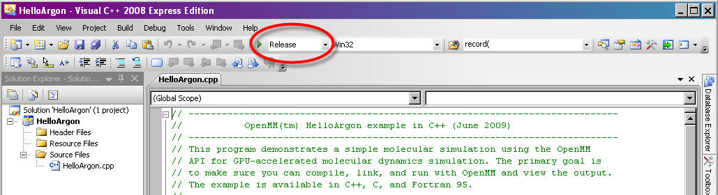
Figure 10-1: Setting “Solution Configuration” to “Release” mode in Visual Studio
From the command options select Debug -> Start Without Debugging (or CTRL-F5). See Figure 10-2. This will also compile the program, if it has not previously been compiled.
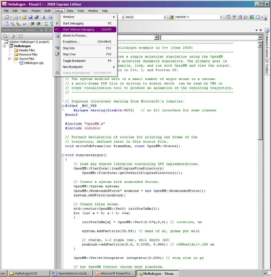
Figure 10-2: Run a program in Visual Studio
You should see a series of lines like the following output on your screen:
REMARK  Using OpenMM platform Reference
MODEL     1
ATOM      1  AR   AR     1       0.000   0.000   0.000  1.00  0.00
ATOM      2  AR   AR     1       5.000   0.000   0.000  1.00  0.00
ATOM      3  AR   AR     1       10.000  0.000   0.000  1.00  0.00
ENDMDL

…

MODEL     250
ATOM      1  AR   AR     1       0.233   0.000   0.000  1.00  0.00
ATOM      2  AR   AR     1       5.068   0.000   0.000  1.00  0.00
ATOM      3  AR   AR     1       9.678   0.000   0.000  1.00  0.00
ENDMDL
MODEL     251
ATOM      1  AR   AR     1       0.198   0.000   0.000  1.00  0.00
ATOM      2  AR   AR     1       5.082   0.000   0.000  1.00  0.00
ATOM      3  AR   AR     1       9.698   0.000   0.000  1.00  0.00
ENDMDL
MODEL     252
ATOM      1  AR   AR     1       0.165   0.000   0.000  1.00  0.00
ATOM      2  AR   AR     1       5.097   0.000   0.000  1.00  0.00
ATOM      3  AR   AR     1       9.717   0.000   0.000  1.00  0.00
ENDMDL
10.2.1.1. Determining the platform being used
The very first line of the output will indicate whether you are running on the CPU (Reference platform) or a GPU (CUDA or OpenCL platform). It will say one of the following:
REMARK  Using OpenMM platform Reference
REMARK  Using OpenMM platform Cuda
REMARK  Using OpenMM platform OpenCL
If you have a supported GPU, the program should, by default, run on the GPU.
10.2.1.2. Visualizing the results
You can output the results to a PDB file that could be visualized using programs like VMD (http://www.ks.uiuc.edu/Research/vmd/) or PyMol (http://pymol.sourceforge.net/). To do this within Visual Studios:
Right-click on the project name HelloArgon (not one of the files) and select the “Properties” option.
On the “Property Pages” form, select “Debugging” under the “Configuration Properties” node.
In the “Command Arguments” field, type:
> argon.pdb
This will save the output to a file called argon.pdb in the current working directory (default is the VisualStudio directory). If you want to save it to another directory, you will need to specify the full path.
Select “OK”
Now, when you run the program in Visual Studio, no text will appear. After a short time, you should see the message “Press any key to continue…,” indicating that the program is complete and that the PDB file has been completely written.
10.2.2. Mac OS X/Linux
Navigate to wherever you saved the example files.
Verify your makefile by consulting the MakefileNotes file in this directory, if necessary.
Type::
make
Then run the program by typing:
./HelloArgon
You should see a series of lines like the following output on your screen:
REMARK  Using OpenMM platform Reference
MODEL     1
ATOM      1  AR   AR     1       0.000   0.000   0.000  1.00  0.00
ATOM      2  AR   AR     1       5.000   0.000   0.000  1.00  0.00
ATOM      3  AR   AR     1       10.000  0.000   0.000  1.00  0.00
ENDMDL

...

MODEL     250
ATOM      1  AR   AR     1       0.233   0.000   0.000  1.00  0.00
ATOM      2  AR   AR     1       5.068   0.000   0.000  1.00  0.00
ATOM      3  AR   AR     1       9.678   0.000   0.000  1.00  0.00
ENDMDL
MODEL     251
ATOM      1  AR   AR     1       0.198   0.000   0.000  1.00  0.00
ATOM      2  AR   AR     1       5.082   0.000   0.000  1.00  0.00
ATOM      3  AR   AR     1       9.698   0.000   0.000  1.00  0.00
ENDMDL
MODEL     252
ATOM      1  AR   AR     1       0.165   0.000   0.000  1.00  0.00
ATOM      2  AR   AR     1       5.097   0.000   0.000  1.00  0.00
ATOM      3  AR   AR     1       9.717   0.000   0.000  1.00  0.00
ENDMDL
10.2.2.1. Determining the platform being used
The very first line of the output will indicate whether you are running on the CPU (Reference platform) or a GPU (CUDA or OpenCL platform). It will say one of the following:
REMARK  Using OpenMM platform Reference
REMARK  Using OpenMM platform Cuda
REMARK  Using OpenMM platform OpenCL
If you have a supported GPU, the program should, by default, run on the GPU.
10.2.2.2. Visualizing the results
You can output the results to a PDB file that could be visualized using programs like VMD (http://www.ks.uiuc.edu/Research/vmd/) or PyMol (http://pymol.sourceforge.net/) by typing:
./HelloArgon > argon.pdb
10.2.2.3. Compiling Fortran and C examples
The Makefile provided with the examples can also be used to compile the Fortran and C examples.
The Fortran compiler needs to load a version of the libstdc++.dylib library that is compatible with the version of gcc used to build OpenMM; OpenMM for Mac is compiled using gcc 4.2. If you are compiling with a different version, edit the Makefile and add the following flag to FCPPLIBS: –L/usr/lib/gcc/i686 -apple-darwin10/4.2.1.
When the Makefile has been updated, type:
make all
10.3. HelloArgon Program
The HelloArgon program simulates three argon atoms in a vacuum. It is a simple program primarily intended for you to verify that you are able to compile, link, and run with OpenMM. It also demonstrates the basic calls needed to run a simulation using OpenMM.
10.3.1. Including OpenMM-defined functions
The OpenMM header file OpenMM.h instructs the program to include everything defined by the OpenMM libraries. Include the header file by adding the following line at the top of your program:
#include "OpenMM.h"
10.3.2. Running a program on GPU platforms
By default, a program will run on the Reference platform. In order to run a program on another platform (e.g., an NVIDIA or AMD GPU), you need to load the required shared libraries for that other platform (e.g., Cuda, OpenCL). The easy way to do this is to call:
OpenMM::Platform::loadPluginsFromDirectory(OpenMM::Platform::getDefaultPluginsDirectory());
This will load all the shared libraries (plug-ins) that can be found, so you do not need to explicitly know which libraries are available on a given machine. In this way, the program will be able to run on another platform, if it is available.
10.3.3. Running a simulation using the OpenMM public API
The OpenMM public API was described in Section 8.5. Here you will see how to use those classes to create a simple system of three argon atoms and run a short simulation. The main components of the simulation are within the function simulateArgon():
System – We first establish a system and add a non-bonded force to it. At this point, there are no particles in the system.
// Create a system with nonbonded forces.
OpenMM::System system;
OpenMM::NonbondedForce* nonbond = new OpenMM::NonbondedForce();
system.addForce(nonbond);
We then add the three argon atoms to the system. For this system, all the data for the particles are hard-coded into the program. While not a realistic scenario, it makes the example simpler and clearer. The std::vector<OpenMM::Vec3> is an array of vectors of 3.
// Create three atoms.
std::vector<OpenMM::Vec3> initPosInNm(3);
for (int a = 0; a < 3; ++a)
{
    initPosInNm[a] = OpenMM::Vec3(0.5*a,0,0); // location, nm

    system.addParticle(39.95); // mass of Ar, grams per mole

    // charge, L-J sigma (nm), well depth (kJ)
    nonbond->addParticle(0.0, 0.3350, 0.996); // vdWRad(Ar)=.188 nm
}
Units: Be very careful with the units in your program. It is very easy to make mistakes with the units, so we recommend including them in your variable names, as we have done here initPosInNm (position in nanometers). OpenMM provides conversion constants that should be used whenever there are conversions to be done; for simplicity, we did not do that in HelloArgon, but all the other examples show the use of these constants.
It is hard to overemphasize the importance of careful units handling—it is very easy to make a mistake despite, or perhaps because of, the trivial nature of units conversion. For more information about the units used in OpenMM, see Section 18.2.
Adding Particle Information: Both the system and the non-bonded force require information about the particles. The system just needs to know the mass of the particle. The non-bonded force requires information about the charge (in this case, argon is uncharged), and the Lennard-Jones parameters sigma (zero-energy separation distance) and well depth (see Section 19.6.1 for more details).
Note that the van der Waals radius for argon is 0.188 nm and that it has already been converted to sigma (0.335 nm) in the example above where it is added to the non-bonded force; in your code, you should make use of the appropriate conversion factor supplied with OpenMM as discussed in Section 18.2.
Integrator – We next specify the integrator to use to perform the calculations. In this case, we choose a Verlet integrator to run a constant energy simulation. The only argument required is the step size in picoseconds.
OpenMM::VerletIntegrator integrator(0.004); // step size in ps
We have chosen to use 0.004 picoseconds, or 4 femtoseconds, which is larger than that used in a typical molecular dynamics simulation. However, since this example does not have any bonds with higher frequency components, like most molecular dynamics simulations do, this is an acceptable value.
Context – The context is an object that consists of an integrator and a system. It manages the state of the simulation. The code below initializes the context. We then let the context select the best platform available to run on, since this is not specifically specified, and print out the chosen platform. This is useful information, especially when debugging.
// Let OpenMM Context choose best platform.
OpenMM::Context context(system, integrator);
printf("REMARK  Using OpenMM platform %s\n", context.getPlatform().getName().c_str());
We then initialize the system, setting the initial time, as well as the initial positions and velocities of the atoms. In this example, we leave time and velocity at their default values of zero.
// Set starting positions of the atoms. Leave time and velocity zero.
context.setPositions(initPosInNm);
Initialize and run the simulation – The next block of code runs the simulation and saves its output. For each frame of the simulation (in this example, a frame is defined by the advancement interval of the integrator; see below), the current state of the simulation is obtained and written out to a PDB-formatted file.
// Simulate.
for (int frameNum=1; ;++frameNum) {
    // Output current state information.
    OpenMM::State state = context.getState(OpenMM::State::Positions);
    const double  timeInPs = state.getTime();
    writePdbFrame(frameNum, state); // output coordinates
Getting state information has to be done in bulk, asking for information for all the particles at once. This is computationally expensive since this information can reside on the GPUs and requires communication overhead to retrieve, so you do not want to do it very often. In the above code, we only request the positions, since that is all that is needed, and time from the state.
The simulation stops after 10 ps; otherwise we ask the integrator to take 10 steps (so one frame is equivalent to 10 time steps). Normally, we would want to take more than 10 steps at a time, but to get a reasonable-looking animation, we use 10.
if (timeInPs >= 10.)
    break;

// Advance state many steps at a time, for efficient use of OpenMM.
integrator.step(10); // (use a lot more than this normally)
10.3.4. Error handling for OpenMM
Error handling for OpenMM is explicitly designed so you do not have to check the status after every call. If anything goes wrong, OpenMM throws an exception. It uses standard exceptions, so on many platforms, you will get the exception message automatically. However, we recommend using try-catch blocks to ensure you do catch the exception.
int main()
{
    try {
        simulateArgon();
        return 0; // success!
    }
    // Catch and report usage and runtime errors detected by OpenMM and fail.
    catch(const std::exception& e) {
        printf("EXCEPTION: %s\n", e.what());
        return 1; // failure!
    }
}
10.3.5. Writing out PDB files
For the HelloArgon program, we provide a simple PDB file writing function writePdbFrame that only writes out argon atoms. The function has nothing to do with OpenMM except for using the OpenMM State. The function extracts the positions from the State in nanometers (10-9 m) and converts them to Angstroms (10-10 m) to be compatible with the PDB format. Again, we emphasize how important it is to track the units being used!
void writePdbFrame(int frameNum, const OpenMM::State& state)
{
    // Reference atomic positions in the OpenMM State.
    const std::vector<OpenMM::Vec3>& posInNm = state.getPositions();

    // Use PDB MODEL cards to number trajectory frames
    printf("MODEL     %d\n", frameNum); // start of frame
    for (int a = 0; a < (int)posInNm.size(); ++a)
    {
        printf("ATOM  %5d  AR   AR     1    ", a+1); // atom number
        printf("%8.3f%8.3f%8.3f  1.00  0.00\n",      // coordinates
        // "*10" converts nanometers to Angstroms
        posInNm[a][0]*10, posInNm[a][1]*10, posInNm[a][2]*10);
    }
    printf("ENDMDL\n"); // end of frame
}
MODEL and ENDMDL are used to mark the beginning and end of a frame, respectively. By including multiple frames in a PDB file, you can visualize the simulation trajectory.
10.3.6. HelloArgon output
The output of the HelloArgon program can be saved to a .pdb file and visualized using programs like VMD or PyMol (see Section 10.2). You should see three atoms moving linearly away and towards one another:

You may need to adjust the van der Waals radius in your visualization program to see the atoms colliding.
10.4. HelloSodiumChloride Program
The HelloSodiumChloride models several sodium (Na+) and chloride (Cl-) ions in implicit solvent (using a Generalized Born/Surface Area, or GBSA, OBC model). As with the HelloArgon program, only non-bonded forces are simulated.
The main purpose of this example is to illustrate our recommended strategy for integrating OpenMM into an existing molecular dynamics (MD) code:
- Write a few, high-level interface routines containing all your OpenMM calls: Rather than make OpenMM calls throughout your program, we recommend writing a handful of interface routines that understand both your MD code’s data structures and OpenMM. Organize these routines into a separate compilation unit so you do not have to make huge changes to your existing MD code. These routines could be written in any language that is callable from the existing MD code. We recommend writing them in C++ since that is what OpenMM is written in, but you can also write them in C or Fortran; see Chapter 12.
- Call only these high-level interface routines from your existing MD code: This provides a clean separation between the existing MD code and OpenMM, so that changes to OpenMM will not directly impact the existing MD code. One way to implement this is to use opaque handles, a standard trick used (for example) for opening files in Linux. An existing MD code can communicate with OpenMM via the handle, but knows none of the details of the handle. It only has to hold on to the handle and give it back to OpenMM.
In the example described below, you will see how this strategy can be implemented for a very simple MD code. Chapter 13 describes the strategies used in integrating OpenMM into real MD codes.
10.4.1. Simple molecular dynamics system
The initial sections of HelloSodiumChloride.cpp represent a very simple molecular dynamics system. The system includes modeling and simulation parameters and the atom and force field data. It also provides a data structure posInAng[3] for storing the current state. These sections represent (in highly simplified form) information that would be available from an existing MD code, and will be used to demonstrate how to integrate OpenMM with an existing MD program.
// -----------------------------------------------------------------
//                   MODELING AND SIMULATION PARAMETERS
// -----------------------------------------------------------------
static const double Temperature         = 300;     // Kelvins
static const double FrictionInPerPs     = 91.;     // collisions per picosecond
static const double SolventDielectric   = 80.;     // typical for water
static const double SoluteDielectric    = 2.;      // typical for protein

static const double StepSizeInFs        = 2;       // integration step size (fs)
static const double ReportIntervalInFs  = 50;      // how often to issue PDB frame (fs)
static const double SimulationTimeInPs  = 100;     // total simulation time (ps)

// Decide whether to request energy calculations.
static const bool   WantEnergy          = true;


// -----------------------------------------------------------------
//                          ATOM AND FORCE FIELD DATA
// -----------------------------------------------------------------
// This is not part of OpenMM; just a struct we can use to collect atom
// parameters for this example. Normally atom parameters would come from the
// force field's parameterization file. We're going to use data in Angstrom and
// Kilocalorie units and show how to safely convert to OpenMM's internal unit
// system which uses nanometers and kilojoules.
static struct MyAtomInfo {
    const char* pdb;
    double      mass, charge, vdwRadiusInAng, vdwEnergyInKcal,
                gbsaRadiusInAng, gbsaScaleFactor;
    double      initPosInAng[3];
    double      posInAng[3]; // leave room for runtime state info
} atoms[] = {
// pdb   mass  charge  vdwRad vdwEnergy   gbsaRad gbsaScale  initPos
{" NA ", 22.99,  1,    1.8680, 0.00277,    1.992,   0.8,     8, 0,  0},
{" CL ", 35.45, -1,    2.4700, 0.1000,     1.735,   0.8,    -8, 0,  0},
{" NA ", 22.99,  1,    1.8680, 0.00277,    1.992,   0.8,     0, 9,  0},
{" CL ", 35.45, -1,    2.4700, 0.1000,     1.735,   0.8,     0,-9,  0},
{" NA ", 22.99,  1,    1.8680, 0.00277,    1.992,   0.8,     0, 0,-10},
{" CL ", 35.45, -1,    2.4700, 0.1000,     1.735,   0.8,     0, 0, 10},
{""} // end of list
};
10.4.2. Interface routines
The key to our recommended integration strategy is the interface routines. You will need to decide what interface routines are required for effective communication between your existing MD program and OpenMM, but typically there will only be six or seven. In our example, the following four routines suffice:
- Initialize: Data structures that already exist in your MD program (i.e., force fields, constraints, atoms in the system) are passed to the Initialize routine, which makes appropriate calls to OpenMM and then returns a handle to the OpenMM object that can be used by the existing MD program.
- Terminate: Clean up the heap space allocated by Initialize by passing the handle to the Terminate routine.
- Advance State: The AdvanceState routine advances the simulation. It requires that the calling function, the existing MD code, gives it a handle.
- Retrieve State: When you want to do an analysis or generate some kind of report, you call the RetrieveState routine. You have to give it a handle. It then fills in a data structure that is defined in the existing MD code, allowing the MD program to use it in its existing routines without further modification.
Note that these are just descriptions of the routines’ functions—you can call them anything you like and implement them in whatever way makes sense for your MD code.
In the example code, the four routines performing these functions, plus an opaque data structure (the handle), would be declared, as shown below. Then, the main program, which sets up, runs, and reports on the simulation, accesses these routines and the opaque data structure (in this case, the variable omm). As you can see, it does not have access to any OpenMM declarations, only to the interface routines that you write so there is no need to change the build environment.
struct MyOpenMMData;
static MyOpenMMData* myInitializeOpenMM(const MyAtomInfo atoms[],
                                        double temperature,
                                        double frictionInPs,
                                        double solventDielectric,
                                        double soluteDielectric,
                                        double stepSizeInFs,
                                        std::string& platformName);
static void          myStepWithOpenMM(MyOpenMMData*, int numSteps);
static void          myGetOpenMMState(MyOpenMMData*,
                                      bool wantEnergy,
                                      double& time,
                                      double& energy,
                                      MyAtomInfo atoms[]);
static void          myTerminateOpenMM(MyOpenMMData*);


// -----------------------------------------------------------------
//                                MAIN PROGRAM
// -----------------------------------------------------------------
int main() {
    const int NumReports     = (int)(SimulationTimeInPs*1000 / ReportIntervalInFs + 0.5);
    const int NumSilentSteps = (int)(ReportIntervalInFs / StepSizeInFs + 0.5);

    // ALWAYS enclose all OpenMM calls with a try/catch block to make sure that
    // usage and runtime errors are caught and reported.
    try {
        double        time, energy;
        std::string   platformName;

        // Set up OpenMM data structures; returns OpenMM Platform name.
        MyOpenMMData* omm = myInitializeOpenMM(atoms, Temperature, FrictionInPerPs,
             SolventDielectric, SoluteDielectric, StepSizeInFs, platformName);

        // Run the simulation:
        //  (1) Write the first line of the PDB file and the initial configuration.
        //  (2) Run silently entirely within OpenMM between reporting intervals.
        //  (3) Write a PDB frame when the time comes.
        printf("REMARK  Using OpenMM platform %s\n", platformName.c_str());
        myGetOpenMMState(omm, WantEnergy, time, energy, atoms);
        myWritePDBFrame(1, time, energy, atoms);

        for (int frame=2; frame <= NumReports; ++frame) {
            myStepWithOpenMM(omm, NumSilentSteps);
            myGetOpenMMState(omm, WantEnergy, time, energy, atoms);
            myWritePDBFrame(frame, time, energy, atoms);
        }

        // Clean up OpenMM data structures.
        myTerminateOpenMM(omm);

        return 0; // Normal return from main.
    }

    // Catch and report usage and runtime errors detected by OpenMM and fail.
    catch(const std::exception& e) {
        printf("EXCEPTION: %s\n", e.what());
        return 1;
    }
}
We will examine the implementation of each of the four interface routines and the opaque data structure (handle) in the sections below.
10.4.2.1. Units
The simple molecular dynamics system described in Section 10.4.1 employs the commonly used units of angstroms and kcals. These differ from the units and parameters used within OpenMM (see Section 18.2): nanometers and kilojoules. These differences may be small but they are critical and must be carefully accounted for in the interface routines.
10.4.2.2. Lennard-Jones potential
The Lennard-Jones potential describes the energy between two identical atoms as the distance between them varies.
The van der Waals “size” parameter is used to identify the distance at which the energy between these two atoms is at a minimum (that is, where the van der Waals force is most attractive). There are several ways to specify this parameter, typically, either as the van der Waals radius rvdw or as the actual distance between the two atoms dmin (also called rmin), which is twice the van der Waals radius rvdw. A third way to describe the potential is through sigma \(\sigma\), which identifies the distance at which the energy function crosses zero as the atoms move closer together than dmin. (See Section 19.6.1 for more details about the relationship between these).
\(\sigma\) turns out to be about 0.89*dmin, which is close enough to dmin that it makes it hard to distinguish the two. Be very careful that you use the correct value. In the example below, we will show you how to use the built-in OpenMM conversion constants to avoid errors.
Lennard-Jones parameters are defined for pairs of identical atoms, but must also be applied to pairs of dissimilar atoms. That is done by “combining rules” that differ among popular MD codes. Two of the most common are:
- Lorentz-Berthelot (used by AMBER, CHARMM):
- Jorgensen (used by OPLS):
where r = the effective van der Waals “size” parameter (minimum radius, minimum distance, or zero crossing (sigma)), and \(\epsilon\) = the effective van der Waals energy well depth parameter, for the dissimilar pair of atoms i and j.
OpenMM only implements Lorentz-Berthelot directly, but others can be implemented using the CustomNonbondedForce class. (See Section 20.4 for details.)
10.4.2.3. Opaque handle MyOpenMMData
In this example, the handle used by the interface to OpenMM is a pointer to a struct called MyOpenMMData. The pointer itself is opaque, meaning the calling program has no knowledge of what the layout of the object it points to is, or how to use it to directly interface with OpenMM. The calling program will simply pass this opaque handle from one interface routine to another.
There are many different ways to implement the handle. The code below shows just one example. A simulation requires three OpenMM objects (a System, a Context, and an Integrator) and so these must exist within the handle. If other objects were required for a simulation, you would just add them to your handle; there would be no change in the main program using the handle.
struct MyOpenMMData {
    MyOpenMMData() : system(0), context(0), integrator(0) {}
    ~MyOpenMMData() {delete system; delete context; delete integrator;}
    OpenMM::System*         system;
    OpenMM::Context*        context;
    OpenMM::Integrator*     integrator;
};
In addition to establishing pointers to the required three OpenMM objects, MyOpenMMData has a constructor MyOpenMMData() that sets the pointers for the three OpenMM objects to zero and a destructor ~MyOpenMMData() that (in C++) gives the heap space back. This was done in-line in the HelloArgon program, but we recommend you use something like the method here instead.
10.4.2.4. myInitializeOpenMM
The myInitializeOpenMM function takes the data structures and simulation parameters from the existing MD code and returns a new handle that can be used to do efficient computations with OpenMM. It also returns the platformName so the calling program knows what platform (e.g., CUDA, OpenCL, Reference) was used.
static MyOpenMMData*
myInitializeOpenMM( const MyAtomInfo    atoms[],
                    double              temperature,
                    double              frictionInPs,
                    double              solventDielectric,
                    double              soluteDielectric,
                    double              stepSizeInFs,
                    std::string&        platformName)
This initialization routine is very similar to the HelloArgon example program, except that objects are created and put in the handle. For instance, just as in the HelloArgon program, the first step is to load the OpenMM plug-ins, so that the program will run on the best performing platform that is available. Then, a System is created and assigned to the handle omm. Similarly, forces are added to the System which is already in the handle.
// Load all available OpenMM plugins from their default location.
OpenMM::Platform::loadPluginsFromDirectory
       (OpenMM::Platform::getDefaultPluginsDirectory());

// Allocate space to hold OpenMM objects while we're using them.
MyOpenMMData* omm = new MyOpenMMData();

// Create a System and Force objects within the System. Retain a reference
// to each force object so we can fill in the forces. Note: the OpenMM
// System takes ownership of the force objects;don't delete them yourself.
omm->system = new OpenMM::System();
OpenMM::NonbondedForce* nonbond = new OpenMM::NonbondedForce();
OpenMM::GBSAOBCForce*   gbsa    = new OpenMM::GBSAOBCForce();
omm->system->addForce(nonbond);
omm->system->addForce(gbsa);

// Specify dielectrics for GBSA implicit solvation.
gbsa->setSolventDielectric(solventDielectric);
gbsa->setSoluteDielectric(soluteDielectric);
In the next step, atoms are added to the System within the handle, with information about each atom coming from the data structure that was passed into the initialization function from the existing MD code. As shown in the HelloArgon program, both the System and the forces need information about the atoms. For those unfamiliar with the C++ Standard Template Library, the push_back function called at the end of this code snippet just adds the given argument to the end of a C++ “vector” container.
// Specify the atoms and their properties:
//  (1) System needs to know the masses.
//  (2) NonbondedForce needs charges,van der Waals properties(in MD units!).
//  (3) GBSA needs charge, radius, and scale factor.
//  (4) Collect default positions for initializing the simulation later.
std::vector<Vec3> initialPosInNm;
for (int n=0; *atoms[n].pdb; ++n) {
     const MyAtomInfo& atom = atoms[n];

     omm->system->addParticle(atom.mass);

     nonbond->addParticle(atom.charge,
                         atom.vdwRadiusInAng * OpenMM::NmPerAngstrom
                                             * OpenMM::SigmaPerVdwRadius,
                         atom.vdwEnergyInKcal * OpenMM::KJPerKcal);

     gbsa->addParticle(atom.charge,
                       atom.gbsaRadiusInAng * OpenMM::NmPerAngstrom,
                       atom.gbsaScaleFactor);

     // Convert the initial position to nm and append to the array.
     const Vec3 posInNm(atom.initPosInAng[0] * OpenMM::NmPerAngstrom,
                  atom.initPosInAng[1] * OpenMM::NmPerAngstrom,
                  atom.initPosInAng[2] * OpenMM::NmPerAngstrom);
     initialPosInNm.push_back(posInNm);
Units: Here we emphasize the need to pay special attention to the units. As mentioned earlier, the existing MD code in this example uses units of angstroms and kcals, but OpenMM uses nanometers and kilojoules. So the initialization routine will need to convert the values from the existing MD code into the OpenMM units before assigning them to the OpenMM objects.
In the code above, we have used the unit conversion constants that come with OpenMM (e.g., OpenMM::NmPerAngstrom) to perform these conversions. Combined with the naming convention of including the units in the variable name (e.g., initPosInAng), the unit conversion constants are useful reminders to pay attention to units and minimize errors.
Finally, the initialization routine creates the Integrator and Context for the simulation. Again, note the change in units for the arguments! The routine then gets the platform that will be used to run the simulation and returns that, along with the handle omm, back to the calling function.
// Choose an Integrator for advancing time, and a Context connecting the
// System with the Integrator for simulation. Let the Context choose the
// best available Platform. Initialize the configuration from the default
// positions we collected above. Initial velocities will be zero but could
// have been set here.
omm->integrator = new OpenMM::LangevinIntegrator(temperature,
frictionInPs,
stepSizeInFs * OpenMM::PsPerFs);
omm->context    = new OpenMM::Context(*omm->system, *omm->integrator);
omm->context->setPositions(initialPosInNm);

platformName = omm->context->getPlatform().getName();
return omm;
10.4.2.5. myGetOpenMMState
The myGetOpenMMState function takes the handle and returns the time, energy, and data structure for the atoms in a way that the existing MD code can use them without modification.
static void
myGetOpenMMState(MyOpenMMData* omm, bool wantEnergy,
                 double& timeInPs, double& energyInKcal, MyAtomInfo atoms[])
Again, this is another interface routine in which you need to be very careful of your units! Note the conversion from the OpenMM units back to the units used in the existing MD code.
int infoMask = 0;
infoMask = OpenMM::State::Positions;
if (wantEnergy) {
   infoMask += OpenMM::State::Velocities; // for kinetic energy (cheap)
   infoMask += OpenMM::State::Energy;     // for pot. energy (more expensive)
}
// Forces are also available (and cheap).

const OpenMM::State state = omm->context->getState(infoMask);
timeInPs = state.getTime(); // OpenMM time is in ps already

// Copy OpenMM positions into atoms array and change units from nm to Angstroms.
const std::vector<Vec3>& positionsInNm = state.getPositions();
for (int i=0; i < (int)positionsInNm.size(); ++i)
    for (int j=0; j < 3; ++j)
         atoms[i].posInAng[j] = positionsInNm[i][j] * OpenMM::AngstromsPerNm;

// If energy has been requested, obtain it and convert from kJ to kcal.
energyInKcal = 0;
if (wantEnergy)
   energyInKcal = (state.getPotentialEnergy() + state.getKineticEnergy())
                  * OpenMM::KcalPerKJ;
10.4.2.6. myStepWithOpenMM
The myStepWithOpenMM routine takes the handle, uses it to find the Integrator, and then sets the number of steps for the Integrator to take. It does not return any values.
static void
myStepWithOpenMM(MyOpenMMData* omm, int numSteps) {
    omm->integrator->step(numSteps);
}
10.4.2.7. myTerminateOpenMM
The myTerminateOpenMM routine takes the handle and deletes all the components, e.g., the Context and System, cleaning up the heap space.
static void
myTerminateOpenMM(MyOpenMMData* omm) {
    delete omm;
}
10.5. HelloEthane Program
The HelloEthane program simulates ethane (H3-C-C-H3) in a vacuum. It is structured similarly to the HelloSodiumChloride example, but includes bonded forces (bond stretch, bond angle bend, dihedral torsion). In setting up these bonded forces, the program illustrates some of the other inconsistencies in definitions and units that you should watch out for.
The bonded forces are added to the system within the initialization interface routine, similar to how the non-bonded forces were added in the HelloSodiumChloride example:
// Create a System and Force objects within the System. Retain a reference
// to each force object so we can fill in the forces. Note: the System owns
// the force objects and will take care of deleting them; don't do it yourself!
OpenMM::System&                 system      = *(omm->system = new OpenMM::System());
OpenMM::NonbondedForce&         nonbond     = *new OpenMM::NonbondedForce();
OpenMM::HarmonicBondForce&      bondStretch = *new OpenMM::HarmonicBondForce();
OpenMM::HarmonicAngleForce&     bondBend    = *new OpenMM::HarmonicAngleForce();
OpenMM::PeriodicTorsionForce&   bondTorsion = *new OpenMM::PeriodicTorsionForce();
system.addForce(&nonbond);
system.addForce(&bondStretch);
system.addForce(&bondBend);
system.addForce(&bondTorsion);
Constrainable and non-constrainable bonds: In the initialization routine, we also set up the bonds. If constraints are being used, then we tell the System about the constrainable bonds:
std::vector< std::pair<int,int> > bondPairs;
for (int i=0; bonds[i].type != EndOfList; ++i) {
    const int*      atom = bonds[i].atoms;
    const BondType& bond = bondType[bonds[i].type];

    if (UseConstraints && bond.canConstrain) {
        system.addConstraint(atom[0], atom[1],
                bond.nominalLengthInAngstroms * OpenMM::NmPerAngstrom);
    }
Otherwise, we need to give the HarmonicBondForce the bond stretch parameters.
Warning: The constant used to specify the stiffness may be defined differently between the existing MD code and OpenMM. For instance, AMBER uses the constant, as given in the harmonic energy term kx2, where the force is 2kx (k = constant and x = distance). OpenMM wants the constant, as used in the force term kx (with energy 0.5 * kx2). So a factor of 2 must be introduced when setting the bond stretch parameters in an OpenMM system using data from an AMBER system.
bondStretch.addBond(atom[0], atom[1], bond.nominalLengthInAngstroms * OpenMM::NmPerAngstrom,
                    bond.stiffnessInKcalPerAngstrom2 * 2 * OpenMM::KJPerKcal *
                    OpenMM::AngstromsPerNm * OpenMM::AngstromsPerNm);
Non-bond exclusions: Next, we deal with non-bond exclusions. These are used for pairs of atoms that appear close to one another in the network of bonds in a molecule. For atoms that close, normal non-bonded forces do not apply or are reduced in magnitude. First, we create a list of bonds to generate the non- bond exclusions:
bondPairs.push_back(std::make_pair(atom[0], atom[1]));
OpenMM’s non-bonded force provides a convenient routine for creating the common exceptions. These are: (1) for atoms connected by one bond (1-2) or connected by just one additional bond (1-3), Coulomb and van der Waals terms do not apply; and (2) for atoms connected by three bonds (1-4), Coulomb and van der Waals terms apply but are reduced by a force-field dependent scale factor. In general, you may introduce additional exceptions, but the standard ones suffice here and in many other circumstances.
// Exclude 1-2, 1-3 bonded atoms from nonbonded forces, and scale down 1-4 bonded atoms.
nonbond.createExceptionsFromBonds(bondPairs, Coulomb14Scale, LennardJones14Scale);

// Create the 1-2-3 bond angle harmonic terms.
for (int i=0; angles[i].type != EndOfList; ++i) {
     const int*       atom  = angles[i].atoms;
     const AngleType& angle = angleType[angles[i].type];

// See note under bond stretch above regarding the factor of 2 here.
bondBend.addAngle(atom[0],atom[1],atom[2],
angle.nominalAngleInDegrees     * OpenMM::RadiansPerDegree,
angle.stiffnessInKcalPerRadian2 * 2 *
OpenMM::KJPerKcal);
}

// Create the 1-2-3-4 bond torsion (dihedral) terms.
for (int i=0; torsions[i].type != EndOfList; ++i) {
     const int*         atom = torsions[i].atoms;
    const TorsionType& torsion = torsionType[torsions[i].type];
    bondTorsion.addTorsion(atom[0],atom[1],atom[2],atom[3],
            torsion.periodicity,
            torsion.phaseInDegrees  * OpenMM::RadiansPerDegree,
            torsion.amplitudeInKcal * OpenMM::KJPerKcal);
}
The rest of the code is similar to the HelloSodiumChloride example and will not be covered in detail here. Please refer to the program HelloEthane.cpp itself, which is well-commented, for additional details.
11. Platform-Specific Properties
When creating a Context, you can specify values for properties specific to a particular Platform. This is used to control how calculations are done in ways that are outside the scope of the generic OpenMM API.
To do this, pass both the Platform object and a map of property values to the Context constructor:
Platform& platform = Platform::getPlatformByName("OpenCL");
map<string, string> properties;
properties["OpenCLDeviceIndex"] = "1";
Context context(system, integrator, platform, properties);
After a Context is created, you can use the Platform’s getPropertyValue() method to query the values of properties.
11.1. OpenCL Platform
The OpenCL Platform recognizes the following Platform-specific properties:
- OpenCLPrecision: This selects what numeric precision to use for calculations. The allowed values are “single”, “mixed”, and “double”. If it is set to “single”, nearly all calculations are done in single precision. This is the fastest option but also the least accurate. If it is set to “mixed”, forces are computed in single precision but integration is done in double precision. This gives much better energy conservation with only a slight decrease in speed. If it is set to “double”, all calculations are done in double precision. This is the most accurate option, but is usually much slower than the others.
- OpenCLUseCpuPme: This selects whether to use the CPU-based PME implementation. The allowed values are “true” or “false”. Depending on your hardware, this might (or might not) improve performance. To use this option, you must have FFTW (single precision, multithreaded) installed, and your CPU must support SSE 4.1.
- OpenCLPlatformIndex: When multiple OpenCL implementations are installed on your computer, this is used to select which one to use. The value is the zero-based index of the platform (in the OpenCL sense, not the OpenMM sense) to use, in the order they are returned by the OpenCL platform API. This is useful, for example, in selecting whether to use a GPU or CPU based OpenCL implementation.
- OpenCLDeviceIndex: When multiple OpenCL devices are available on your computer, this is used to select which one to use. The value is the zero-based index of the device to use, in the order they are returned by the OpenCL device API.
The OpenCL Platform also supports parallelizing a simulation across multiple GPUs. To do that, set the OpenCLDeviceIndex property to a comma separated list of values. For example,
properties["OpenCLDeviceIndex"] = "0,1";
This tells it to use both devices 0 and 1, splitting the work between them.
11.2. CUDA Platform
The CUDA Platform recognizes the following Platform-specific properties:
- CudaPrecision: This selects what numeric precision to use for calculations. The allowed values are “single”, “mixed”, and “double”. If it is set to “single”, nearly all calculations are done in single precision. This is the fastest option but also the least accurate. If it is set to “mixed”, forces are computed in single precision but integration is done in double precision. This gives much better energy conservation with only a slight decrease in speed. If it is set to “double”, all calculations are done in double precision. This is the most accurate option, but is usually much slower than the others.
- CudaUseCpuPme: This selects whether to use the CPU-based PME implementation. The allowed values are “true” or “false”. Depending on your hardware, this might (or might not) improve performance. To use this option, you must have FFTW (single precision, multithreaded) installed, and your CPU must support SSE 4.1.
- CudaCompiler: This specifies the path to the CUDA kernel compiler. If you do
not specify this, OpenMM will try to locate the compiler itself. Specify this
only when you want to override the default location. The logic used to pick the
default location depends on the operating system:
- Mac/Linux: It first looks for an environment variable called OPENMM_CUDA_COMPILER. If that is set, its value is used. Otherwise, the default location is set to /usr/local/cuda/bin/nvcc.
- Windows: It looks for an environment variable called CUDA_BIN_PATH, then appends nvcc.exe to it. That environment variable is set by the CUDA installer, so it usually is present.
- CudaTempDirectory: This specifies a directory where temporary files can be written while compiling kernels. OpenMM usually can locate your operating system’s temp directory automatically (for example, by looking for the TEMP environment variable), so you rarely need to specify this.
- CudaDeviceIndex: When multiple CUDA devices are available on your computer, this is used to select which one to use. The value is the zero-based index of the device to use, in the order they are returned by the CUDA API.
- CudaUseBlockingSync: This is used to control how the CUDA runtime synchronizes between the CPU and GPU. If this is set to “true” (the default), CUDA will allow the calling thread to sleep while the GPU is performing a computation, allowing the CPU to do other work. If it is set to “false”, CUDA will spin-lock while the GPU is working. Setting it to “false” can improve performance slightly, but also prevents the CPU from doing anything else while the GPU is working.
The CUDA Platform also supports parallelizing a simulation across multiple GPUs. To do that, set the CudaDeviceIndex property to a comma separated list of values. For example,
properties["CudaDeviceIndex"] = "0,1";
This tells it to use both devices 0 and 1, splitting the work between them.
11.3. CPU Platform
The CPU Platform recognizes the following Platform-specific properties:
CpuThreads: This specifies the number of CPU threads to use. If you do not specify this, OpenMM will select a default number of threads as follows:
- If an environment variable called OPENMM_CPU_THREADS is set, its value is used as the number of threads.
- Otherwise, the number of threads is set to the number of logical CPU cores in the computer it is running on.
Usually the default value works well. This is mainly useful when you are running something else on the computer at the same time, and you want to prevent OpenMM from monopolizing all available cores.
12. Using OpenMM with Software Written in Languages Other than C++
Although the native OpenMM API is object-oriented C++ code, it is possible to directly translate the interface so that it is callable from C, Fortran 95, and Python with no substantial conceptual changes. We have developed a straightforward mapping for these languages that, while perhaps not the most elegant possible, has several advantages:
- Almost all documentation, training, forum discussions, and so on are equally useful to users of all these languages. There are syntactic differences of course, but all the important concepts remain unchanged.
- We are able to generate the C, Fortran, and Python APIs from the C++ API. Obviously, this reduces development effort, but more importantly it means that the APIs are likely to be error-free and are always available immediately when the native API is updated.
- Because OpenMM performs expensive operations “in bulk” there is no noticeable overhead in accessing these operations through the C, Fortran, or Python APIs.
- All symbols introduced to a C or Fortran program begin with the prefix “OpenMM_” so will not interfere with symbols already in use.
Availability of APIs in other languages: All necessary C and Fortran bindings are built in to the main OpenMM library; no separate library is required. The Python wrappers are contained in a module that is distributed with OpenMM and that can be installed by executing its setup.py script in the standard way.
(This doesn’t apply to most users: if you are building your own OpenMM from source using CMake and want the API bindings generated, be sure to enable the OPENMM_BUILD_C_AND_FORTRAN_WRAPPERS option for C and Fortran, or OPENMM_BUILD_PYTHON_WRAPPERS option for Python. The Python module will be placed in a subdirectory of your main build directory called “python”)
Documentation for APIs in other languages: While there is extensive Doxygen documentation available for the C++ and Python APIs, there is no separate on-line documentation for the C and Fortran API. Instead, you should use the C++ documentation, employing the mappings described here to figure out the equivalent syntax in C or Fortran.
12.1. C API
Before you start writing your own C program that calls OpenMM, be sure you can build and run the two C examples that are supplied with OpenMM (see Chapter 10). These can be built from the supplied Makefile on Linux and Mac, or supplied NMakefile and Visual Studio solution files on Windows.
The example programs are HelloArgonInC and HelloSodiumChlorideInC. The argon example serves as a quick check that your installation is set up properly and you know how to build a C program that is linked with OpenMM. It will also tell you whether OpenMM is executing on the GPU or is running (slowly) on the Reference platform. However, the argon example is not a good template to follow for your own programs. The sodium chloride example, though necessarily simplified, is structured roughly in the way we recommended you set up your own programs to call OpenMM. Please be sure you have both of these programs executing successfully on your machine before continuing.
12.1.1. Mechanics of using the C API
The C API is generated automatically from the C++ API when OpenMM is built. There are two resulting components: C bindings (functions to call), and C declarations (in a header file). The C bindings are small extern (global) interface functions, one for every method of every OpenMM class, whose signatures (name and arguments) are predictable from the class name and method signatures. There are also “helper” types and functions provided for the few cases in which the C++ behavior cannot be directly mapped into C. These interface and helper functions are compiled in to the main OpenMM library so there is nothing special you have to do to get access to them.
In the include subdirectory of your OpenMM installation directory, there is a machine-generated header file OpenMMCWrapper.h that should be #included in any C program that is to make calls to OpenMM functions. That header contains declarations for all the OpenMM C interface functions and related types. Note that if you follow our suggested structure, you will not need to include this file in your main() compilation unit but can instead use it only in a local file that you write to provide a simple interface to your existing code (see Chapter 10).
12.1.2. Mapping from the C++ API to the C API
The automated generator of the C “wrappers” follows the translation strategy shown in Table 12-1. The idea is that if you see the construct on the left in the C++ API documentation, you should interpret it as the corresponding construct on the right in C. Please look at the supplied example programs to see how this is done in practice.
| Construct | C++ API declaration | Equivalent in C API |
|---|---|---|
| namespace | OpenMM:: | OpenMM_ (prefix) |
| class | class OpenMM::ClassName | typedef OpenMM_ClassName |
| constant | OpenMM::RadiansPerDeg | OpenMM_RadiansPerDeg (static constant) |
| class enum | OpenMM::State::Positions | OpenMM_State_Positions |
| constructor | new OpenMM::ClassName() | OpenMM_ClassName* OpenMM_ClassName_create()
(additional constructors are _create_2(), etc.)
|
| destructor | OpenMM::ClassName* thing;
delete thing;
|
OpenMM_ClassName* thing;
OpenMM_ClassName_destroy(thing);
|
| class method | OpenMM::ClassName* thing;
thing->method(args);
|
OpenMM_ClassName* thing;
OpenMM_ClassName_method(thing, args)
|
| Boolean (type & constants) | bool
true, false
|
OpenMM_Boolean
OpenMM_True(1), OpenMM_False(0)
|
| string | std::string | char* |
| 3-vector | OpenMM::Vec3 | typedef OpenMM_Vec3 |
| arrays | std::vector<std::string>
std::vector<double>
std::vector<Vec3>
std::vector<std::pair<int,int>>
std::map<std::string,double>
|
typedef OpenMM_StringArray
typedef OpenMM_DoubleArray
typedef OpenMM_Vec3Array
typedef OpenMM_BondArray
typedef OpenMM_ParameterArray
|
Table 12-1: Default mapping of objects from the C++ API to the C API There are some exceptions to the generic translation rules shown in the table; they are enumerated in the next section. And because there are no C++ API equivalents to the array types, they are described in detail below.
12.1.3. Exceptions
These two methods are handled somewhat differently in the C API than in the C++ API:
- OpenMM::Context::getState() The C version, OpenMM_Context_getState(), returns a pointer to a heap allocated OpenMM_State object. You must then explicitly destroy this State object when you are done with it, by calling OpenMM_State_destroy().
- OpenMM::Platform::loadPluginsFromDirectory() The C version OpenMM_Platform_loadPluginsFromDirectory() returns a heap-allocated OpenMM_StringArray object containing a list of all the file names that were successfully loaded. You must then explicitly destroy this StringArray object when you are done with it. Do not ignore the return value; if you do you’ll have a memory leak since the StringArray will still be allocated.
(In the C++ API, the equivalent methods return references into existing memory rather than new heap-allocated memory, so the returned objects do not need to be destroyed.)
12.1.4. OpenMM_Vec3 helper type
Unlike the other OpenMM objects which are opaque and manipulated via pointers, the C API provides an explicit definition for the C OpenMM_Vec3 type that is compatible with the OpenMM::Vec3 type. The definition of OpenMM_Vec3 is:
typedef struct {double x, y, z;} OpenMM_Vec3;
You can work directly with the individual fields of this type from your C program if you want. For convenience, a scale() function is provided that creates a new OpenMM_Vec3 from an old one and a scale factor:
OpenMM_Vec3 OpenMM_Vec3_scale(const OpenMM_Vec3 vec, double scale);
12.1.5. Array helper types
C++ has built-in container types std::vector and std::map which OpenMM uses to manipulate arrays of objects. These don’t have direct equivalents in C, so we supply special array types for each kind of object for which OpenMM creates containers. These are: string, double, Vec3, bond, and parameter map. See Table 12-2 for the names of the C types for each of these object arrays. Each of the array types provides these functions (prefixed by OpenMM_ and the actual Thing name), with the syntax shown conceptually since it differs slightly for each kind of object.
| Function | Operation |
|---|---|
| ThingArray* create(int size) | Create a heap-allocated array of Things, with space pre-allocated to hold size of them. You can start at size==0 if you want since these arrays are dynamically resizeable. |
| void destroy(ThingArray*) | Free the heap space that is currently in use for the passed-in array of Things. |
| int getSize(ThingArray*) | Return the current number of Things in this array. This means you can get() and set() elements up to getSize()-1. |
| void resize(ThingArray*, int size) | Change the size of this array to the indicated value which may be smaller or larger than the current size. Existing elements remain in their same locations as long as they still fit. |
| void append(ThingArray*, Thing) | Add a Thing to the end of the array, increasing the array size by one. The precise syntax depends on the actual type of Thing; see below. |
| void set(ThingArray*, int index, Thing) | Store a copy of Thing in the indicated element of the array (indexed from 0). The array must be of length at least index+1; you can’t grow the array with this function. |
| Thing get(ThingArray*, int index) | Retrieve a particular element from the array (indexed from 0). (For some Things the value is returned in arguments rather than as the function return.) |
Table 12-2: Generic description of array helper types
Here are the exact declarations with deviations from the generic description noted, for each of the array types.
12.1.5.1. OpenMM_DoubleArray
OpenMM_DoubleArray*
            OpenMM_DoubleArray_create(int size);
void        OpenMM_DoubleArray_destroy(OpenMM_DoubleArray*);
int         OpenMM_DoubleArray_getSize(const OpenMM_DoubleArray*);
void        OpenMM_DoubleArray_resize(OpenMM_DoubleArray*, int size);
void        OpenMM_DoubleArray_append(OpenMM_DoubleArray*, double value);
void        OpenMM_DoubleArray_set(OpenMM_DoubleArray*, int index, double value);
double      OpenMM_DoubleArray_get(const OpenMM_DoubleArray*, int index);
12.1.5.2. OpenMM_StringArray
OpenMM_StringArray*
            OpenMM_StringArray_create(int size);
void        OpenMM_StringArray_destroy(OpenMM_StringArray*);
int         OpenMM_StringArray_getSize(const OpenMM_StringArray*);
void        OpenMM_StringArray_resize(OpenMM_StringArray*, int size);
void        OpenMM_StringArray_append(OpenMM_StringArray*, const char* string);
void        OpenMM_StringArray_set(OpenMM_StringArray*, int index, const char* string);
const char* OpenMM_StringArray_get(const OpenMM_StringArray*, int index);
12.1.5.3. OpenMM_Vec3Array
OpenMM_Vec3Array*
            OpenMM_Vec3Array_create(int size);
void        OpenMM_Vec3Array_destroy(OpenMM_Vec3Array*);
int         OpenMM_Vec3Array_getSize(const OpenMM_Vec3Array*);
void        OpenMM_Vec3Array_resize(OpenMM_Vec3Array*, int size);
void        OpenMM_Vec3Array_append(OpenMM_Vec3Array*, const OpenMM_Vec3 vec);
void        OpenMM_Vec3Array_set(OpenMM_Vec3Array*, int index, const OpenMM_Vec3 vec);
const OpenMM_Vec3*
            OpenMM_Vec3Array_get(const OpenMM_Vec3Array*, int index);
12.1.5.4. OpenMM_BondArray
Note that bonds are specified by pairs of integers (the atom indices). The get() method returns those in a pair of final arguments rather than as its functional return.
OpenMM_BondArray*
            OpenMM_BondArray_create(int size);
void        OpenMM_BondArray_destroy(OpenMM_BondArray*);
int         OpenMM_BondArray_getSize(const OpenMM_BondArray*);
void        OpenMM_BondArray_resize(OpenMM_BondArray*, int size);
void        OpenMM_BondArray_append(OpenMM_BondArray*, int particle1, int particle2);
void        OpenMM_BondArray_set(OpenMM_BondArray*, int index, int particle1, int particle2);
void        OpenMM_BondArray_get(const OpenMM_BondArray*, int index,
                                 int* particle1, int* particle2);
12.1.5.5. OpenMM_ParameterArray
OpenMM returns references to internal ParameterArrays but does not support user-created ParameterArrays, so only the get() and getSize() functions are available. Also, note that since this is actually a map rather than an array, the “index” is the name of the parameter rather than its ordinal.
int         OpenMM_ParameterArray_getSize(const OpenMM_ParameterArray*);
double      OpenMM_ParameterArray_get(const OpenMM_ParameterArray*, const char* name);
12.2. Fortran 95 API
Before you start writing your own Fortran program that calls OpenMM, be sure you can build and run the two Fortran examples that are supplied with OpenMM (see Chapter 10). These can be built from the supplied Makefile on Linux and Mac, or supplied NMakefile and Visual Studio solution files on Windows.
The example programs are HelloArgonInFortran and HelloSodiumChlorideInFortran. The argon example serves as a quick check that your installation is set up properly and you know how to build a Fortran program that is linked with OpenMM. It will also tell you whether OpenMM is executing on the GPU or is running (slowly) on the Reference platform. However, the argon example is not a good template to follow for your own programs. The sodium chloride example, though necessarily simplified, is structured roughly in the way we recommended you set up your own programs to call OpenMM. Please be sure you have both of these programs executing successfully on your machine before continuing.
12.2.1. Mechanics of using the Fortran API
The Fortran API is generated automatically from the C++ API when OpenMM is built. There are two resulting components: Fortran bindings (subroutines to call), and Fortran declarations of types and subroutines (in the form of a Fortran 95 module file). The Fortran bindings are small interface subroutines, one for every method of every OpenMM class, whose signatures (name and arguments) are predictable from the class name and method signatures. There are also “helper” types and subroutines provided for the few cases in which the C++ behavior cannot be directly mapped into Fortran. These interface and helper subroutines are compiled in to the main OpenMM library so there is nothing special you have to do to get access to them.
Because Fortran is case-insensitive, calls to Fortran subroutines (however capitalized) are mapped by the compiler into all-lowercase or all-uppercase names, and different compilers use different conventions. The automatically-generated OpenMM Fortran “wrapper” subroutines, which are generated in C and thus case-sensitive, are provided in two forms for compatibility with the majority of Fortran compilers, including Intel Fortran and gfortran. The two forms are: (1) all-lowercase with a trailing underscore, and (2) all-uppercase without a trailing underscore. So regardless of the Fortran compiler you are using, it should find a suitable subroutine to call in the main OpenMM library.
In the include subdirectory of your OpenMM installation directory, there is a machine-generated module file OpenMMFortranModule.f90 that must be compiled along with any Fortran program that is to make calls to OpenMM functions. (You can look at the Makefile or Visual Studio solution file provided with the OpenMM examples to see how to build a program that uses this module file.) This module file contains definitions for two modules: MODULE OpenMM_Types and MODULE OpenMM; however, only the OpenMM module will appear in user programs (it references the other module internally). The modules contain declarations for all the OpenMM Fortran interface subroutines, related types, and parameters (constants). Note that if you follow our suggested structure, you will not need to use the OpenMM module in your main() compilation unit but can instead use it only in a local file that you write to provide a simple interface to your existing code (see Chapter 10).
12.2.2. Mapping from the C++ API to the Fortran API
The automated generator of the Fortran “wrappers” follows the translation strategy shown in Table 12-3. The idea is that if you see the construct on the left in the C++ API documentation, you should interpret it as the corresponding construct on the right in Fortran. Please look at the supplied example programs to see how this is done in practice. Note that all subroutines and modules are declared with “implicit none”, meaning that the type of every symbol is declared explicitly and should not be inferred from the first letter of the symbol name.
| Construct | C++ API declaration | Equivalent in Fortran API |
|---|---|---|
| namespace | OpenMM:: | OpenMM_ (prefix) |
| class | class OpenMM::ClassName | type (OpenMM_ClassName) |
| constant | OpenMM::RadiansPerDeg | parameter (OpenMM_RadiansPerDeg) |
| class enum | OpenMM::State::Positions | parameter (OpenMM_State_Positions) |
| constructor | new OpenMM::ClassName() | type (OpenMM_ClassName) thing
call OpenMM_ClassName_create(thing)
(additional constructors are _create_2(), etc.)
|
| destructor | OpenMM::ClassName* thing;
delete thing;
|
type (OpenMM_ClassName) thing
call OpenMM_ClassName_destroy(thing)
|
| class method | OpenMM::ClassName* thing;
thing->method(args*)
|
type (OpenMM_ClassName) thing
call OpenMM_ClassName_method(thing, args)
|
| Boolean (type & constants) | bool
true
false
|
integer*4
parameter (OpenMM_True=1)
parameter (OpenMM_False=0)
|
| string | std::string | character(*) |
| 3-vector | OpenMM::Vec3 | real*8 vec(3) |
| arrays | std::vector<std::string> std::vector<double> std::vector<Vec3> std::vector<std::pair<int,int>> std::map<std::string, double> | type (OpenMM_StringArray)
type (OpenMM_DoubleArray)
type (OpenMM_Vec3Array)
type (OpenMM_BondArray)
type (OpenMM_ParameterArray)
|
Table 12-3: Default mapping of objects from the C++ API to the Fortran API
Because there are no C++ API equivalents to the array types, they are described in detail below.
12.2.3. OpenMM_Vec3 helper type
Unlike the other OpenMM objects which are opaque and manipulated via pointers, the Fortran API uses an ordinary real*8(3) array in place of the OpenMM::Vec3 type. You can work directly with the individual elements of this type from your Fortran program if you want. For convenience, a scale() function is provided that creates a new Vec3 from an old one and a scale factor:
subroutine OpenMM_Vec3_scale(vec, scale, result)
real*8 vec(3), scale, result(3)
No explicit type(OpenMM_Vec3) is provided in the Fortran API since it is not needed.
12.2.4. Array helper types
C++ has built-in container types std::vector and std::map which OpenMM uses to manipulate arrays of objects. These don’t have direct equivalents in Fortran, so we supply special array types for each kind of object for which OpenMM creates containers. These are: string, double, Vec3, bond, and parameter map. See Table 12-4 for the names of the Fortran types for each of these object arrays. Each of the array types provides these functions (prefixed by OpenMM_ and the actual Thing name), with the syntax shown conceptually since it differs slightly for each kind of object.
| Function | Operation |
|---|---|
subroutine create(array,size)
type (OpenMM_ThingArray) array
integer*4 size
|
Create a heap-allocated array of Things, with space pre-allocated to hold size of them. You can start at size==0 if you want since these arrays are dynamically resizeable. |
subroutine destroy(array)
type (OpenMM_ThingArray) array
|
Free the heap space that is currently in use for the passed-in array of Things. |
function getSize(array)
type (OpenMM_ThingArray) array
integer*4 size
|
Return the current number of Things in this array. This means you can get() and set() elements up to getSize(). |
subroutine resize(array,size)
type (OpenMM_ThingArray) array
integer*4 size
|
Change the size of this array to the indicated value which may be smaller or larger than the current size. Existing elements remain in their same locations as long as they still fit. |
subroutine append(array,elt)
type (OpenMM_ThingArray) array
Thing elt
|
Add a Thing to the end of the array, increasing the array size by one. The precise syntax depends on the actual type of Thing; see below. |
subroutine set(array,index,elt)
type (OpenMM_ThingArray) array
integer*4 size
Thing elt
|
Store a copy of elt in the indicated element of the array (indexed from 1). The array must be of length at least index; you can’t grow the array with this function. |
subroutine get(array,index,elt)
type (OpenMM_ThingArray) array
integer*4 size
Thing elt
|
Retrieve a particular element from the array (indexed from 1). Some Things require more than one argument to return. |
Table 12-4: Generic description of array helper types
Here are the exact declarations with deviations from the generic description noted, for each of the array types.
12.2.4.1. OpenMM_DoubleArray
subroutine OpenMM_DoubleArray_create(array, size)
    integer*4 size
    type (OpenMM_DoubleArray) array
subroutine OpenMM_DoubleArray_destroy(array)
    type (OpenMM_DoubleArray) array
function OpenMM_DoubleArray_getSize(array)
    type (OpenMM_DoubleArray) array
    integer*4 OpenMM_DoubleArray_getSize
subroutine OpenMM_DoubleArray_resize(array, size)
    type (OpenMM_DoubleArray) array
    integer*4 size
subroutine OpenMM_DoubleArray_append(array, value)
    type (OpenMM_DoubleArray) array
    real*8 value
subroutine OpenMM_DoubleArray_set(array, index, value)
    type (OpenMM_DoubleArray) array
    integer*4 index
    real*8 value
subroutine OpenMM_DoubleArray_get(array, index, value)
    type (OpenMM_DoubleArray) array
    integer*4 index
    real*8 value
12.2.4.2. OpenMM_StringArray
subroutine OpenMM_StringArray_create(array, size)
    integer*4 size
    type (OpenMM_StringArray) array
subroutine OpenMM_StringArray_destroy(array)
    type (OpenMM_StringArray) array
function OpenMM_StringArray_getSize(array)
    type (OpenMM_StringArray) array
    integer*4 OpenMM_StringArray_getSize
subroutine OpenMM_StringArray_resize(array, size)
    type (OpenMM_StringArray) array
    integer*4 size
subroutine OpenMM_StringArray_append(array, str)
    type (OpenMM_StringArray) array
    character(*) str
subroutine OpenMM_StringArray_set(array, index, str)
    type (OpenMM_StringArray) array
    integer*4 index
    character(*) str
subroutine OpenMM_StringArray_get(array, index, str)
    type (OpenMM_StringArray) array
    integer*4 index
    character(*)str
12.2.4.3. OpenMM_Vec3Array
subroutine OpenMM_Vec3Array_create(array, size)
    integer*4 size
    type (OpenMM_Vec3Array) array
subroutine OpenMM_Vec3Array_destroy(array)
    type (OpenMM_Vec3Array) array
function OpenMM_Vec3Array_getSize(array)
    type (OpenMM_Vec3Array) array
    integer*4 OpenMM_Vec3Array_getSize
subroutine OpenMM_Vec3Array_resize(array, size)
    type (OpenMM_Vec3Array) array
    integer*4 size
subroutine OpenMM_Vec3Array_append(array, vec)
    type (OpenMM_Vec3Array) array
    real*8 vec(3)
subroutine OpenMM_Vec3Array_set(array, index, vec)
    type (OpenMM_Vec3Array) array
    integer*4 index
    real*8 vec(3)
subroutine OpenMM_Vec3Array_get(array, index, vec)
    type (OpenMM_Vec3Array) array
    integer*4 index
    real*8 vec (3)
12.2.4.4. OpenMM_BondArray
Note that bonds are specified by pairs of integers (the atom indices). The get() method returns those in a pair of final arguments rather than as its functional return.
subroutine OpenMM_BondArray_create(array, size)
    integer*4 size
    type (OpenMM_BondArray) array
subroutine OpenMM_BondArray_destroy(array)
    type (OpenMM_BondArray) array
function OpenMM_BondArray_getSize(array)
    type (OpenMM_BondArray) array
    integer*4 OpenMM_BondArray_getSize
subroutine OpenMM_BondArray_resize(array, size)
    type (OpenMM_BondArray) array
    integer*4 size
subroutine OpenMM_BondArray_append(array, particle1, particle2)
    type (OpenMM_BondArray) array
    integer*4 particle1, particle2
subroutine OpenMM_BondArray_set(array, index, particle1, particle2)
    type (OpenMM_BondArray) array
    integer*4 index, particle1, particle2
subroutine OpenMM_BondArray_get(array, index, particle1, particle2)
    type (OpenMM_BondArray) array
    integer*4 index, particle1, particle2
12.2.4.5. OpenMM_ParameterArray
OpenMM returns references to internal ParameterArrays but does not support user-created ParameterArrays, so only the get() and getSize() functions are available. Also, note that since this is actually a map rather than an array, the “index” is the name of the parameter rather than its ordinal.
function OpenMM_ParameterArray_getSize(array)
    type (OpenMM_ParameterArray) array
    integer*4 OpenMM_ParameterArray_getSize
subroutine OpenMM_ParameterArray_get(array, name, param)
    type (OpenMM_ParameterArray) array
    character(*) name
    character(*) param
12.3. Python API
12.3.1. Installing the Python API
There are currently two types of packages for installing the Python API. One contains wrapper source code for Unix-type machines (including Linux and Mac operating systems). You will need a C++ compiler to install it using this type of package. The other type of installation package is a binary package which contains compiled wrapper code for Windows machines (no compilers are needed to install binary packages).
12.3.1.1. Installing on Windows
OpenMM on Windows only works with Python 3.3, so make sure that version is installed before you try installing. For Python installation packages and instructions, go to http://python.org. Note that if you have a 64-bit machine, you should still install the 32-bit version of Python since the OpenMM Python API binary is 32-bit. We suggest that you install Python using the default options.
Double click on the Python API Installer icon, located in the top level directory for the OpenMM installation (by default, this is C:Program FilesOpenMM). This will install the OpenMM package into the Python installation area. If you have more than one Python installation, you will be asked which Python to use—make sure to select Python 3.3.
12.3.1.2. Installing on Linux and Mac
Make sure you have Python 2.6 or later installed. For Python installation packages and instructions, go to http://python.org. If you do not have the correct Python version, install a valid version using the default options. Most versions of Linux and Mac OS X have a suitable Python preinstalled. You can check by typing “python --version” in a terminal window.
You must have a C++ compiler to install the OpenMM Python API. If you are using a Mac, install Apple’s Xcode development tools (http://developer.apple.com/TOOLS/Xcode) to get the needed compiler. On other Unix-type systems, install gcc or clang.
The install.sh script installs the Python API automatically as part of the installation process, so you probably already have it installed. If for some reason you need to install it manually, you can do that with the setup.py script included with OpenMM. Before executing this script, you must set two environment variables: OPENMM_INCLUDE_PATH must point to the directory containing OpenMM header files, and OPENMM_LIB_PATH must point to the directory containing OpenMM library files. Assuming OpenMM is installed in the default location (/usr/local/openmm), you would type the following commands. Note that if you are using the system Python (as opposed to a locally installed version), you may need to use the sudo command when running python setup.py install.
export OPENMM_INCLUDE_PATH=/usr/local/openmm/include
export OPENMM_LIB_PATH=/usr/local/openmm/lib
python setup.py build
python setup.py install
If you are compiling OpenMM from source, you can also install by building the “PythonInstall” target:
make PythonInstall OR sudo make PythonInstall
12.3.2. Mapping from the C++ API to the Python API
The Python API follows the C++ API as closely as possible. There are three notable differences:
The getState() method in the Context class takes Pythonic-type arguments to indicate which state variables should be made available. For example:
myContext.getState(getEnergy=True, getForce=False, …)
Wherever the C++ API uses references to return multiple values from a method, the Python API returns a tuple. For example, in C++ you would query a HarmonicBondForce for a bond’s parameters as follows:
int particle1, particle2;
double length, k;
f.getBondParameters(i, particle1, particle2, length, k);
In Python, the equivalent code is:
[particle1, particle2, length, k] = f.getBondParameters(i)
Unlike C++, the Python API accepts and returns quantities with units attached to most values (see Section 12.3.4 below for details). In short, this means that while values in C++ have implicit units, the Python API returns objects that have values and explicit units.
12.3.3. Mechanics of using the Python API
When using the Python API, be sure to include the GPU support libraries in your library path, just as you would for a C++ application. This is set with the LD_LIBRARY_PATH environment variable on Linux, DYLD_LIBRARY_PATH on Mac, or PATH on Windows. See Chapter 3 for details.
The Python API is contained in the simtk.openmm package, while the units code is contained in the simtk.units package. (The application layer, described in the Application Guide, is contained in the simtk.openmm.app package.) A program using it will therefore typically begin
import simtk.openmm as mm
import simtk.unit as unit
Creating and using OpenMM objects is then done exactly as in C++:
system = mm.System()
nb = mm.NonbondedForce()
nb.setNonbondedMethod(mm.NonbondedForce.CutoffNonPeriodic)
nb.setCutoffDistance(1.2*unit.nanometer)
system.addForce(nb)
Note that when setting the cutoff distance, we explicitly specify that it is in nanometers. We could just as easily specify it in different units:
nb.setCutoffDistance(12*unit.angstrom)
The use of units in OpenMM is discussed in the next section.
12.3.4. Units and dimensional analysis
12.3.4.1. Why does the Python API include units?
The C++ API for OpenMM uses an implicit set of units for physical quantities such as lengths, masses, energies, etc. These units are based on daltons, nanometers, and picoseconds for the mass, length, and time dimensions, respectively. When using the C++ API, it is very important to ensure that quantities being manipulated are always expressed in terms of these units. For example, if you read in a distance in Angstroms, you must multiply that distance by a conversion factor to turn it into nanometers before using it in the C++ API. Such conversions can be a source of tedium and errors. This is true in many areas of scientific programming. Units confusion was blamed for the loss of the Mars Climate Orbiter spacecraft in 1999, at a cost of more than $100 million. Units were introduced in the Python API to minimize the chance of such errors.
The Python API addresses the potential problem of conversion errors by using quantities with explicit units. If a particular distance is expressed in Angstroms, the Python API will know that it is in Angstroms. When the time comes to call the C++ API, it will understand that the quantity must be converted to nanometers. You, the programmer, must declare upfront that the quantity is in Angstrom units, and the API will take care of the details from then on. Using explicit units is a bit like brushing your teeth: it requires some effort upfront, but it probably saves you trouble in the long run.
12.3.4.2. Quantities, units, and dimensions
The explicit unit system is based on three concepts: Dimensions, Units, and Quantities.
Dimensions are measurable physical concepts such as mass, length, time, and energy. Energy is actually a composite dimension based on mass, length, and time.
A Unit defines a linear scale used to measure amounts of a particular physical Dimension. Examples of units include meters, seconds, joules, inches, and grams.
A Quantity is a specific amount of a physical Dimension. An example of a quantity is “0.63 kilograms”. A Quantity is expressed as a combination of a value (e.g., 0.63), and a Unit (e.g., kilogram). The same Quantity can be expressed in different Units.
The set of BaseDimensions defined in the simtk.unit module includes:
- mass
- length
- time
- temperature
- amount
- charge
- luminous intensity
These are not precisely the same list of base dimensions used in the SI unit system. SI defines “current” (charge per time) as a base unit, while simtk.unit uses “charge”. And simtk.unit treats angle as a dimension, even though angle quantities are often considered dimensionless. In this case, we choose to err on the side of explicitness, particularly because interconversion of degrees and radians is a frequent source of unit headaches.
12.3.4.3. Units examples
Many common units are defined in the simtk.unit module.
from simtk.unit import nanometer, angstrom, dalton
Sometimes you don’t want to type the full unit name every time, so you can assign it a shorter name using the as functionality:
from simtk.unit import nanometer as nm
New quantities can be created from a value and a unit. You can use either the multiply operator (‘*’) or the explicit Quantity constructor:
from simk.unit import nanometer, Quantity
# construct a Quantity using the multiply operator
bond_length = 1.53 * nanometer
# equivalently using the explicit Quantity constructor
bond_length = Quantity(1.53, nanometer)
# or more verbosely
bond_length = Quantity(value=1.53, unit=nanometer)
When working with Numpy arrays you must use the explicit constructor. You cannot multiply them by a unit, because the Numpy array class overloads the multiply operator.
12.3.4.4. Arithmetic with units
Addition and subtraction of quantities is only permitted between quantities that share the same dimension. It makes no sense to add a mass to a distance. If you attempt to add or subtract two quantities with different dimensions, an exception will be raised. This is a good thing; it helps you avoid errors.
x = 5.0*dalton + 4.3*nanometer; # error
Addition or subtraction of quantities with the same dimension, but different units, is fine, and results in a new quantity created using the correct conversion factor between the units used.
x = 1.3*nanometer + 5.6*angstrom; # OK, result in nanometers
Quantities can be added and subtracted. Naked Units cannot.
Multiplying or dividing two quantities creates a new quantity with a composite dimension. For example, dividing a distance by a time results in a velocity.
from simtk.unit import kilogram, meter, second
a = 9.8 * meter / second**2; # acceleration
m = 0.36 * kilogram; # mass
F = m * a; # force in kg*m/s**2::
Multiplication or division of two Units results in a composite Unit.
mps = meter / second
Unlike amount (moles), angle (radians) is arguably dimensionless. But simtk.unit treats angle as another dimension. Use the trigonometric functions from the simtk.unit module (not those from the Python math module!) when dealing with Units and Quantities.
from simtk.unit import sin, cos, acos
x = sin(90.0*degrees)
angle = acos(0.68); # returns an angle quantity (in radians)
The method pow() is a built-in Python method that works with Quantities and Units.
area = pow(3.0*meter, 2)
# or, equivalently
area = (3.0*meter)**2
# or
area = 9.0*(meter**2)
The method sqrt() is not as built-in as pow(). Do not use the Python math.sqrt() method with Units and Quantities. Use the simtk.unit.sqrt() method instead:
from simtk.unit import sqrt
side_length = sqrt(4.0*meter**2)
12.3.4.5. Atomic scale mass and energy units are “per amount”
Mass and energy units at the atomic scale are specified “per amount” in the simtk.unit module. Amount (mole) is one of the seven fundamental dimensions in the SI unit system. The atomic scale mass unit, dalton, is defined as grams per mole. The dimension of dalton is therefore mass/amount, instead of simply mass. Similarly, the atomic scale energy unit, kilojoule_per_mole (and kilocalorie_per_mole) has “per amount” in its dimension. Be careful to always use “per amount” mass and energy types at the atomic scale, and your dimensional analysis should work out properly.
The energy unit kilocalories_per_mole does not have the same Dimension as the macroscopic energy unit kilocalories. Molecular scientists sometimes use the word “kilocalories” when they mean “kilocalories per mole”. Use “kilocalories per mole” or”kilojoules per mole” for molecular energies. Use “kilocalories” for the metabolic energy content of your lunch. The energy unit kilojoule_per_mole happens to go naturally with the units nanometer, picoseconds, and dalton. This is because 1 kilojoule/mole happens to be equal to 1 gram-nanometer2/mole-picosecond2, and is therefore consistent with the molecular dynamics unit system used in the C++ OpenMM API.
These “per mole” units are what you should be using for molecular calculations, as long as you are using SI / cgs / calorie sorts of units.
12.3.4.6. SI prefixes
Many units with SI prefixes such as “milligram” (milli) and “kilometer” (kilo) are provided in the simtk.unit module. Others can be created by multiplying a prefix symbol by a non-prefixed unit:
from simtk.unit import mega, kelvin
megakelvin = mega * kelvin
t = 8.3 * megakelvin
Only grams and meters get all of the SI prefixes (from yotto-(10-24) to yotta-(1024)) automatically.
12.3.4.7. Converting to different units
Use the Quantity.in_units_of() method to create a new Quantity with different units.
from simtk.unit import nanosecond, fortnight
x = (175000*nanosecond).in_units_of(fortnight)
When you want a plain number out of a Quantity, use the value_in_unit() method:
from simtk.unit import femtosecond, picosecond
t = 5.0*femtosecond
t_just_a_number = t.value_in_unit(picoseconds)
Using value_in_unit() puts the responsibility for unit analysis back into your hands, and it should be avoided. It is sometimes necessary, however, when you are called upon to use a non-units-aware Python API.
12.3.4.8. Lists, tuples, vectors, numpy arrays, and Units
Units can be attached to containers of numbers to create a vector quantity. The simtk.unit module overloads the __setitem__ and __getitem__ methods for these containers to ensure that Quantities go in and out.
>>> a = Vec3(1,2,3) * nanometers
>>> print(a)
(1, 2, 3) nm
>>> print(a.in_units_of(angstroms))
(10.0, 20.0, 30.0) A

>>> s2 = [[1,2,3],[4,5,6]] * centimeter
>>> print(s2)
[[1, 2, 3], [4, 5, 6]] cm
>>> print(s2/millimeter)
[[10.0, 20.0, 30.0], [40.0, 50.0, 60.0]]

>>> import numpy
>>> a = Quantity(numpy.array([1,2,3]), centimeter)
>>> print(a)
[1 2 3] cm
>>> print(a/millimeter)
[ 10.  20.  30.]
Converting a whole list to different units at once is much faster than converting each element individually. For example, consider the following code that prints out the position of every particle in a State, as measured in Angstroms:
for v in state.getPositions():
    print(v.value_in_unit(angstrom))
This can be rewritten as follows:
for v in state.getPositions().value_in_unit(angstrom):
    print(v)
The two versions produce identical results, but the second one will run faster, and therefore is preferred.
13. Examples of OpenMM Integration
13.1. GROMACS
GROMACS is a large, complex application written primarily in C. The considerations involved in adapting it to use OpenMM are likely to be similar to those faced by developers of other existing applications.
The first principle we followed in adapting GROMACS was to keep all OpenMM-related code isolated to just a few files, while modifying as little of the existing GROMACS code as possible. This minimized the risk of breaking existing parts of the code, while making the OpenMM-related parts as easy to work with as possible. It also minimized the need for C code to invoke the C++ API. (This would not be an issue if we used the OpenMM C API wrapper, but that is less convenient than the C++ API, and placing all of the OpenMM calls into separate C++ files solves the problem equally well.) Nearly all of the OpenMM-specific code is contained in a single file, openmm_wrapper.cpp. It defines four functions which encapsulate all of the interaction between OpenMM and the rest of GROMACS:
openmm_init(): As arguments, this function takes pointers to lots of internal GROMACS data structures that describe the simulation to be run. It creates a System, Integrator, and Context based on them, then returns an opaque reference to an object containing them. That reference is an input argument to all of the other functions defined in openmm_wrapper.cpp. This allows information to be passed between those functions without exposing it to the rest of GROMACS.
openmm_take_one_step(): This calls step(1) on the Integrator that was created by openmm_init().
openmm_copy_state(): This calls getState() on the Context that was created by openmm_init(), and then copies information from the resulting State into various GROMACS data structures. This function is how state data generated by OpenMM is passed back to GROMACS for output, analysis, etc.
openmm_cleanup(): This is called at the end of the simulation. It deletes all the objects that were created by openmm_init().
This set of functions defines the interactions between GROMACS and OpenMM: copying information from the application to OpenMM, performing integration, copying information from OpenMM back to the application, and freeing resources at the end of the simulation. While the details of their implementations are specific to GROMACS, this overall pattern is fairly generic. A similar set of functions can be used for many other applications as well.
13.2. TINKER-OpenMM
TINKER is written primarily in Fortran, and uses common blocks extensively to store application-wide parameters. Rather than modify the TINKER build scripts to allow C++ code, it was decided to use the OpenMM C API instead. Despite these differences, the overall approach used to add OpenMM support was very similar to that used for GROMACS.
TINKER-OpenMM allows OpenMM to be used to calculate forces and energies and to perform the integration in the main molecular dynamics loop. The only changes to the TINKER source code are in the file dynamic.f for the setup and running of a simulation. An added file, dynamic_openmm.c, contains the interface C code between TINKER and OpenMM.
The flow of the molecular dynamics simulation using OpenMM is as follows:
- The TINKER code is used to read the AMOEBA parameter file, the *.xyz and *.key files. It then parses the command-line options.
- The routine map_common_blocks_to_c_data_structs() is called to map the FORTRAN common blocks to C data structures used in setting the parameters used by OpenMM.
- The routine openmm_validate() is called from dynamic.f before the main loop. This routine checks that all required options and settings obtained from the input in step (1) and common blocks in step (2) are available. If an option or setting is unsupported, the program exits with an appropriate message. The routine openmm_validate() and the other OpenMM interface methods are in the file dynamic_openmm.c.
- openmm_init() is called to create the OpenMM System, Integrator and Context objects..
- openmm_take_steps() is called to take a specified number of time steps.
- openmm_update() is then called to retrieve the state (energies/positions/velocities) and populate the appropriate TINKER data structures. These values are converted from the OpenMM units of kJ/nm to kcal/Å when populating the TINKER arrays.
- Once the main loop has completed, the routine openmm_cleanup() is called to delete the OpenMM objects and release resources being used on the GPU.
14. Testing and Validation of OpenMM
The goal of testing and validation is to make sure that OpenMM works correctly. That means that it runs without crashing or otherwise failing, and that it produces correct results. Furthermore, it must work correctly on a variety of hardware platforms (e.g. different models of GPU), software platforms (e.g. operating systems and OpenCL implementations), and types of simulations.
Three types of tests are used to validate OpenMM:
- Unit tests: These are small tests designed to test specific features or pieces of code in isolation. For example, a test of HarmonicBondForce might create a System with just a few particles and bonds, compute the forces and energy, and compare them to the analytically expected values. There are thousands of unit tests that collectively cover all of OpenMM.
- System tests: Whereas unit tests validate small features in isolation, system tests are designed to validate the entire library as a whole. They simulate realistic models of biomolecules and perform tests that are likely to fail if any problem exists anywhere in the library.
- Direct comparison between OpenMM and other programs: The third type of validation performed is a direct comparison of the individual forces computed by OpenMM to those computed by other programs for a collection of biomolecules.
Each type of test is outlined in greater detail below; a discussion of the current status of the tests is then given.
14.1. Description of Tests
14.1.1. Unit tests
The unit tests are with the source code, so if you build from source you can run them yourself. See Section 9.7 for details. When you run the tests (for example, by typing “make test” on Linux or Mac), it should produce output something like this:
      Start   1: TestReferenceAndersenThermostat
1/317 Test   #1: TestReferenceAndersenThermostat .............. Passed  0.26 sec
      Start   2: TestReferenceBrownianIntegrator
2/317 Test   #2: TestReferenceBrownianIntegrator .............. Passed  0.13 sec
      Start   3: TestReferenceCheckpoints
3/317 Test   #3: TestReferenceCheckpoints ..................... Passed  0.02 sec
... <many other tests> ...
Each line represents a test suite, which may contain multiple unit tests. If all tests within a suite passed, it prints the word “Passed” and how long the suite took to execute. Otherwise it prints an error message. If any tests failed, you can then run them individually (each one is a separate executable) to get more details on what went wrong.
14.1.2. System tests
Several different types of system tests are performed. Each type is run for a variety of systems, including both proteins and nucleic acids, and involving both implicit and explicit solvent. The full suite of tests is repeated for both the CUDA and OpenCL platforms, using both single and double precision (and for the integration tests, mixed precision as well), on a variety of operating systems and hardware. There are four types of tests:
- Consistency between platforms: The forces and energy are computed using the platform being tested, then compared to ones computed with the Reference platform. The results are required to agree to within a small tolerance.
- Energy-force consistency: This verifies that the force really is the gradient of the energy. It first computes the vector of forces for a given conformation. It then generates four other conformations by displacing the particle positions by small amounts along the force direction. It computes the energy of each one, uses those to calculate a fourth order finite difference approximation to the derivative along that direction, and compares it to the actual forces. They are required to agree to within a small tolerance.
- Energy conservation: The system is simulated at constant energy using a Verlet integrator, and the total energy is periodically recorded. A linear regression is used to estimate the rate of energy drift. In addition, all constrained distances are monitored during the simulation to make sure they never differ from the expected values by more than the constraint tolerance.
- Thermostability: The system is simulated at constant temperature using a Langevin integrator. The mean kinetic energy over the course of the simulation is computed and compared to the expected value based on the temperature. In addition, all constrained distances are monitored during the simulation to make sure they never differ from the expected values by more than the constraint tolerance.
If you want to run the system tests yourself, they can be found in the Subversion repository at https://simtk.org/svn/pyopenmm/trunk/test/system-tests. Check out that directory, then execute the runAllTests.sh shell script. It will create a series of files with detailed information about the results of the tests. Be aware that running the full test suite may take a long time (possibly several days) depending on the speed of your GPU.
14.1.3. Direct comparisons between OpenMM and other programs
As a final check, identical systems are set up in OpenMM and in another program (Gromacs 4.5 or Tinker 6.1), each one is used to compute the forces on atoms, and the results are directly compared to each other.
14.2. Test Results
In this section, we highlight the major results obtained from the tests described above. They are not exhaustive, but should give a reasonable idea of the level of accuracy you can expect from OpenMM.
14.2.1. Comparison to Reference Platform
The differences between forces computed with the Reference platform and those computed with the OpenCL or CUDA platform are shown in Table 14-1. For every atom, the relative difference between platforms was computed as 2·|Fref–Ftest|/(|Fref|+|Ftest|), where Fref is the force computed by the Reference platform and Ftest is the force computed by the platform being tested (OpenCL or CUDA). The median over all atoms in a given system was computed to estimate the typical force errors for that system. Finally, the median of those values for all test systems was computed to give the value shown in the table.
| Force | OpenCL (single) | OpenCL (double) | CUDA (single) | CUDA (double) |
|---|---|---|---|---|
| Total Force | 2.53·10-6 | 1.44·10-7 | 2.56·10-6 | 8.78·10-8 |
| HarmonicBondForce | 2.88·10-6 | 1.57·10-13 | 2.88·10-6 | 1.57·10-13 |
| HarmonicAngleForce | 2.25·10-5 | 4.21·10-7 | 2.27·10-5 | 4.21·10-7 |
| PeriodicTorsionForce | 8.23·10-7 | 2.44·10-7 | 9.27·10-7 | 2.56·10-7 |
| RBTorsionForce | 4.86·10-6 | 1.46·10-7 | 4.72·10-6 | 1.4·10-8 |
| NonbondedForce (no cutoff) | 1.49·10-6 | 6.49·10-8 | 1.49·10-6 | 6.49·10-8 |
| NonbondedForce (cutoff, nonperiodic) | 9.74·10-7 | 4.88·10-9 | 9.73·10-7 | 4.88·10-9 |
| NonbondedForce (cutoff, periodic) | 9.82·10-7 | 4.88·10-9 | 9.8·10-7 | 4.88·10-9 |
| NonbondedForce (Ewald) | 1.33·10-6 | 5.22·10-9 | 1.33·10-6 | 5.22·10-9 |
| NonbondedForce (PME) | 3.99·10-5 | 4.08·10-6 | 3.99·10-5 | 4.08·10-6 |
| GBSAOBCForce (no cutoff) | 3.0·10-6 | 1.76·10-7 | 3.09·10-6 | 9.4·10-8 |
| GBSAOBCForce (cutoff, nonperiodic) | 2.77·10-6 | 1.76·10-7 | 2.95·10-6 | 9.33·10-8 |
| GBSAOBCForce (cutoff, periodic) | 2.61·10-6 | 1.78·10-7 | 2.77·10-6 | 9.24·10-8 |
Table 14-1: Median relative difference in forces between Reference platform and OpenCL/CUDA platform
14.2.2. Energy Conservation
Figure 14-1 shows the total system energy versus time for three simulations of ubiquitin in OBC implicit solvent. All three simulations used the CUDA platform, a Verlet integrator, a time step of 0.5 fs, no constraints, and no cutoff on the nonbonded interactions. They differ only in the level of numeric precision that was used for calculations (see Chapter 11).
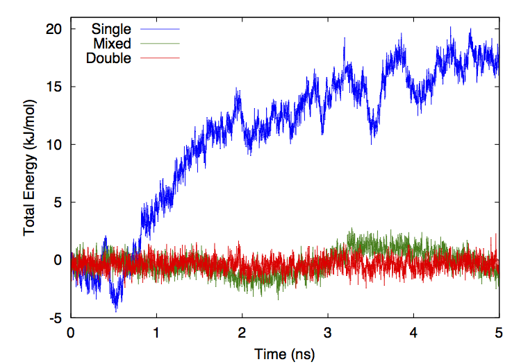
Figure 14-1: Total energy versus time for simulations run in three different precision modes.
For the mixed and double precision simulations, the drift in energy is almost entirely diffusive with negligible systematic drift. The single precision simulation has a more significant upward drift with time, though the rate of drift is still small compared to the rate of short term fluctuations. Fitting a straight line to each curve gives a long term rate of energy drift of 3.98 kJ/mole/ns for single precision, 0.217 kJ/mole/ns for mixed precision, and 0.00100 kJ/mole/ns for double precision. In the more commonly reported units of kT/ns/dof, these correspond to 4.3·10-4 for single precision, 2.3·10-5 for mixed precision, and 1.1·10-7 for double precision.
Be aware that different simulation parameters will give different results. These simulations were designed to minimize all sources of error except those inherent in OpenMM. There are other sources of error that may be significant in other situations. In particular:
- Using a larger time step increases the integration error (roughly proportional to dt2).
- If a system involves constraints, the level of error will depend strongly on the constraint tolerance specified by the Integrator.
- When using Ewald summation or Particle Mesh Ewald, the accuracy will depend strongly on the Ewald error tolerance.
- Applying a distance cutoff to implicit solvent calculations will increase the error, and the shorter the cutoff is, the greater the error will be.
As a result, the rate of energy drift may be much greater in some simulations than in the ones shown above.
14.2.3. Comparison to Gromacs
OpenMM and Gromacs 4.5.5 were each used to compute the atomic forces for dihydrofolate reductase (DHFR) in implicit and explicit solvent. The implicit solvent calculations used the OBC solvent model and no cutoff on nonbonded interactions. The explicit solvent calculations used Particle Mesh Ewald and a 1 nm cutoff on direct space interactions. For OpenMM, the Ewald error tolerance was set to 10-6. For Gromacs, fourierspacing was set to 0.07 and ewald_rtol to 10-6. No constraints were applied to any degrees of freedom. Both programs used single precision. The test was repeated for OpenCL, CUDA, and CPU platforms.
For every atom, the relative difference between OpenMM and Gromacs was computed as 2·|FMM–FGro|/(|FMM|+|FGro|), where FMM is the force computed by OpenMM and FGro is the force computed by Gromacs. The median over all atoms is shown in Table 14-2.
| Solvent Model | OpenCL | CUDA | CPU |
|---|---|---|---|
| Implicit | 7.66·10-6 | 7.68·10-6 | 1.94·10-5 |
| Explicit | 6.77·10-5 | 6.78·10-5 | 9.89·10-5 |
Table 14-2: Median relative difference in forces between OpenMM and Gromacs
15. AMOEBA Plugin
OpenMM 6.2 provides a plugin that implements the AMOEBA polarizable atomic multipole force field from Jay Ponder’s lab. The AMOEBA force field may be used through OpenMM’s Python application layer. We have also created a modified version of TINKER (referred to as TINKER-OpenMM here) that uses OpenMM to accelerate AMOEBA simulations. TINKER-OpenMM can be created from a TINKER package using three files made available through the OpenMM home page. OpenMM AMOEBA Force and System objects containing AMOEBA forces can be serialized.
At present, AMOEBA is only supported on the CUDA and Reference platforms, not on the OpenCL platform.
In the following sections, the individual forces and options available in the plugin are listed, and the steps required to build and use the plugin and TINKER-OpenMM are outlined. Validation results are also reported. Benchmarks can be found on the OpenMM wiki at http://wiki.simtk.org/openmm/Benchmarks.
15.1. OpenMM AMOEBA Supported Forces and Options
15.1.1. Supported Forces and Options
The AMOEBA force terms implemented in OpenMM are listed in Table 15-1 along with the supported and unsupported options. TINKER options that are not supported for any OpenMM force include the grouping of atoms (e.g. protein chains), the infinite polymer check, and no exclusion of particles from energy/force calculations (‘active’/’inactive’ particles). The virial is not calculated for any force.
All rotation axis types are supported: ‘Z-then-X’, ‘Bisector’, ‘Z-Bisect’, ‘3-Fold’, ‘Z-Only’.
| TINKER Force | OpenMM Force | Option/Note |
|---|---|---|
| ebond1 (bondterm) | AmoebaBondForce | bndtyp=’HARMONIC’ supported, ‘MORSE’ not implemented |
| Eangle71 (angleterm) | AmoebaAngleForce | angtyp=’HARMONIC’ and ‘IN-PLANE’ supported; ‘LINEAR’ and ‘FOURIER’ not implemented |
| etors1a (torsionterm) | PeriodicTorsionForce | All options implemented; smoothing version(etors1b) not supported |
| etortor1 (tortorterm) | AmoebaTorsionTorsionForce | All options implemented |
| eopbend1 (opbendterm) | AmoebaOutOfPlaneBendForce | opbtyp = ‘ALLINGER’ implemented; ‘W-D-C’ not implemented |
| epitors1 (pitorsterm) | AmoebaPiTorsionForce | All options implemented |
| estrbnd1 (strbndterm) | AmoebaStretchBendForce | All options implemented |
| ehal1a (vdwterm) | AmoebaVdwForce | ehal1b(LIGHTS) not supported |
| empole1a (mpoleterm) | AmoebaMultipoleForce | poltyp = ‘MUTUAL’, ‘DIRECT’ supported |
| empole1c (mpoleterm) PME | AmoebaMultipoleForce | poltyp = ‘MUTUAL’, ‘DIRECT’ supported; boundary= ‘VACUUM’ unsupported |
| esolv1 (solvateterm) | AmoebaWcaDispersionForce,
AmoebaGeneralizedKirkwoodForce
|
Only born-radius=’grycuk’ and solvate=’GK’ supported; unsupported solvate settings: ‘ASP’, ‘SASA’, ‘ONION’, ‘pb’, ‘GB-HPMF’, ‘Gk-HPMF’; SASA computation is based on ACE approximation |
| eurey1 (ureyterm) | HarmonicBondForce | All options implemented |
Table 15-1: Mapping between TINKER and OpenMM AMOEBA forces
Some specific details to be aware of are the following:
- Forces available in TINKER but not implemented in the OpenMM AMOEBA plugin include the following: angle-angle, out-of-plane distance, improper dihedral, improper torsion, stretch-torsion, charge-charge, atomwise charge-dipole, dipole-dipole, reaction field, ligand field, restraint, scf molecular orbital calculation; strictly speaking, these are not part of the AMOEBA force field.
- Implicit solvent in TINKER-OpenMM is implemented with key file entry ‘solvate GK’. The entry ‘born-radius grycuk’ should also be included; only the ‘grycuk’ option for calculating the Born radii is available in the plugin.
- In TINKER, the nonpolar cavity contribution to the solvation term is calculated using an algorithm that does not map well to GPUs. Instead the OpenMM plugin uses the TINKER version of the ACE approximation to estimate the cavity contribution to the SASA.
- Calculations using the CUDA platform may be done in either single or double precision; for the Reference platform, double precision is used. TINKER uses double precision.
- The TINKER parameter files for the AMOEBA force-field parameters are based on units of kilocalorie/Å, whereas OpenMM uses units of kilojoules/nanometer; both TINKER and OpenMM use picoseconds time units. Hence, in mapping the force-field parameters from TINKER files to OpenMM, many of the parameter values must be converted to the OpenMM units. The setup methods in the TINKER-OpenMM application perform the required conversions.
15.1.2. Supported Integrators
In addition to the limitations to the forces outlined above, TINKER-OpenMM can only use either the ‘Verlet’ or ‘Stochastic’ integrators when the OpenMM plugin is used; an equivalent to the TINKER ‘Beeman’ integrator is unavailable in OpenMM.
15.2. TINKER-OpenMM
15.2.1. Building TINKER-OpenMM (Linux)
Below are instructions for building TINKER-OpenMM in Linux.
To build and install the OpenMM plugin libraries, follow the steps outlined in Chapter 9 (Compiling OpenMM from Source Code). You will need to set the following options to ‘ON’ when you run CMake:
- OPENMM_BUILD_AMOEBA_PLUGIN
- OPENMM_BUILD_AMOEBA_CUDA_LIB
- OPENMM_BUILD_CUDA_LIB
- OPENMM_BUILD_C_AND_FORTRAN_WRAPPERS
Download the complete TINKER distribution from http://dasher.wustl.edu/ffe/ and unzip/untar the file.
Obtain the modified TINKER file dynamic.f, the interface file dynamic_openmm.c and the Makefile from the “Downloads” section of OpenMM’s homepage (https://simtk.org/home/openmm) and place them in the TINKER source directory. These files are compatible with TINKER 6.0.4. If you are using later versions of TINKER, some minor edits may be required to get the program to compile.
In the Makefile, edit the following fields, as needed:
- TINKERDIR – This should point to the head of the TINKER distribution directory, e.g., ‘/home/user/tinker-5.1.09’
- LINKDIR – directory in executable path containing linked copies of the TINKER executables; typical directory would be ‘/usr/local/bin’
- CC – This is an added field that should point to the C compiler (e.g., ‘/usr/bin/gcc’)
- OpenMM_INSTALL_DIR - This should identify the directory where the OpenMM files were installed, i.e., the OPENMM_INSTALL_PREFIX setting when CMake was run in step (1)
At the command line, type:
make dynamic_openmm.x
to create the executable.
Check that the environment variable ‘OPENMM_PLUGIN_DIR’ is set to the installed plugins directory and that the environment variable ‘LD_LIBRARY_PATH’ includes both the installed lib and plugins directory; for example:
OPENMM_PLUGIN_DIR=/home/usr/install/openmm/lib/plugins
LD_LIBRARY_PATH=/usr/local/cuda/lib64:/home/usr/install/openmm/lib:
                /home/usr/install/openmm/lib/plugins
15.2.2. Using TINKER-OpenMM
Run dynamic_openmm.x with the same command-line options as you would dynamic.x. Consult the TINKER documentation and Table 15-1 for more details.
15.2.2.1. Available outputs
Only the total force and potential energy are returned by TINKER-OpenMM; a breakdown of the energy and force into individual terms (bond, angle, …), as is done in TINKER, is unavailable through the OpenMM plugin. Also, the pressure cannot be calculated since the virial is not calculated in the plugin.
15.2.2.2. Setting the frequency of output data updates
Frequent retrieval of the state information from the GPU board can use up a substantial portion of the total wall clock time. This is due to the fact that the forces and energies are recalculated for each retrieval. Hence, if the state information is obtained after every timestep, the wall clock time will approximately double over runs where the state information in only gathered infrequently (say every 50-100 timesteps).
Two options are provided for updating the TINKER data structures:
- (DEFAULT) If the logical value of ‘oneTimeStepPerUpdate’ in dynamic.f is true, then a single step is taken and the TINKER data structures are populated at each step. This option is conceptually simpler and is consistent with the TINKER md loops; for example, the output from the TINKER subroutine mdstat() will be accurate for this choice. However, the performance will be degraded since the forces and energy are recalculated with each call, doubling the required time. This is the default option.
- If ‘oneTimeStepPerUpdate’ is false, then depending on the values of iprint (TINKER keyword ‘PRINTOUT’) and iwrite (=dump time/dt), multiple time steps are taken on the GPU before data is transferred from the GPU to the CPU; here dump time is the value given to the TINKER command-line query ‘Enter Time between Dumps in Picoseconds’. Under this option, every iprint and every iwrite timesteps, the state information will be retrieved. For example if ‘PRINTOUT’ is 10 and iwrite is 15, then the information will be retrieved at time steps { 10, 15, 20, 30, 40, 45, …}. This option will lead to better performance than option 1. However, a downside to this approach is that the fluctuation values printed by the Tinker routine mdstat() will be incorrect.
15.2.2.3. Specify the GPU board to use
To specify a GPU board other than the default, set the environment variable ‘CUDA_DEVICE’ to the desired board id. A line like the following will be printed to stderr for the setting CUDA_DEVICE=2:
Platform Cuda: setting device id to 2 based on env variable CUDA_DEVICE.
15.2.2.4. Running comparison tests between TINKER and OpenMM routines
To turn on testing (comparison of forces and potential energy for the initial conformation calculated using TINKER routines and OpenMM routines), set ‘applyOpenMMTest’ to a non-zero value in dynamic.f. Note: the program exits after the force/energy comparisons; it does not execute the main molecular dynamics loop.
Testing individual forces: An example key file for testing the harmonic bond term is as follows:
parameters /home/user/tinker/params/amoebabio09
verbose
solvate  GK
born-radius  grycuk
polar-eps  0.0001
integrate  verlet
bondterm only
For the other covalent and Van der Waals forces, replace the line bondterm only above with the following lines depending on the force to be tested:
angle force:            angleterm onl
out-of-plane bend:      opbendterm only
stretch bend force      strbndterm only
pi-torsion force:       pitorsterm only
torsion force:          torsionterm only
torsion-torsion force:  tortorterm only
Urey-Bradley force:     ureyterm only
Van der Waals force:    vdwterm only
A sample key file for the multipole force with no cutoffs is given below:
parameters /home/user/tinker/params/amoebabio09
verbose
solvate  GK
born-radius  grycuk
polar-eps  0.0001
integrate  verlet
mpoleterm only
polarizeterm
A sample key file for PME multipole tests
parameters /home/user/tinker/params/amoebabio09
verbose
randomseed  123456789
neighbor-list
vdw-cutoff  12.0
ewald
ewald-cutoff  7.0
pme-grid  64 64 64
polar-eps  0.01
fft-package  fftw
integrate  verlet
mpoleterm only
polarizeterm
For the Generalized Kirkwood force, the following entries are needed:
parameters /home/user/tinker/params/amoebabio09
verbose
solvate  GK
born-radius  grycuk
polar-eps  0.0001
integrate  verlet
solvateterm only
polarizeterm
mpoleterm
For the implicit solvent (‘solvate GK’ runs) test, the forces and energies will differ due to the different treatments of the cavity term (see Section 15.1.1 above). With these options for the Generalized Kirkwood force, the test routine will remove the cavity contribution from the TINKER and OpenMM forces/energy when performing the comparisons between the two calculations.
To test the multipole force or the Generalized Kirkwood forces with direct polarization, add the following line to the end of the above files:
polarization DIRECT
15.2.2.5. Turning off OpenMM / Reverting to TINKER routines
To use the TINKER routines, as opposed to the OpenMM plugin, to run a simulation, set ‘useOpenMM’ to .false. in dynamic.f.
15.3. OpenMM AMOEBA Validation
OpenMM and TINKER 6.1.01 were each used to compute the atomic forces for dihydrofolate reductase (DHFR) in implicit and explicit solvent. Calculations used the CUDA platform, and were repeated for both single and double precision. For every atom, the relative difference between OpenMM and TINKER was computed as 2·|FMM–FT|/(|FMM|+|FT|), where FMM is the force computed by OpenMM and FT is the force computed by TINKER. The median over all atoms is shown in Table 15-2.
Because OpenMM and TINKER use different approximations to compute the cavity term, the differences in forces are much larger for implicit solvent than for explicit solvent. We therefore repeated the calculations, removing the cavity term. This yields much closer agreement between OpenMM and TINKER, demonstrating that the difference comes entirely from that one term.
| Solvent Model | single | double |
|---|---|---|
| Implicit | 1.04·10-2 | 1.04·10-2 |
| Implicit (no cavity term) | 9.23·10-6 | 1.17·10-6 |
| Explicit | 3.73·10-5 | 1.83·10-7 |
Table 15-2: Median relative difference in forces between OpenMM and TINKER
16. Ring Polymer Molecular Dynamics (RPMD) Plugin
Ring Polymer Molecular Dynamics (RPMD) provides an efficient approach to include nuclear quantum effects in molecular simulations.[23] When used to calculate static equilibrium properties, RPMD reduces to path integral molecular dynamics and gives an exact description of the effect of quantum fluctuations for a given potential energy model.[24] For dynamical properties RPMD is no longer exact but has shown to be a good approximation in many cases.
For a system with a classical potential energy E(q), the RPMD Hamiltonian is given by
This Hamiltonian resembles that of a system of classical ring polymers where different copies of the system are connected by harmonic springs. Hence each copy of the classical system is commonly referred to as a “bead”. The spread of the ring polymer representing each particle is directly related to its De Broglie thermal wavelength (uncertainty in its position).
RPMD calculations must be converged with respect to the number n of beads used. Each bead is evolved at the effective temperature nT, where T is the temperature for which properties are required. The number of beads needed to converge a calculation can be estimated using[25]
where \(\omega_{max}\) is the highest frequency in the problem. For example, for flexible liquid water the highest frequency is the OH stretch at around 3000 cm-1, so around 24 to 32 beads are needed depending on the accuracy required. For rigid water where the highest frequency is only around 1000 cm-1, only 6 beads are typically needed. Due to the replication needed of the classical system, the extra cost of the calculation compared to a classical simulation increases linearly with the number of beads used.
This cost can be reduced by “contracting” the ring polymer to a smaller number of beads.[25] The rapidly changing forces are then computed for the full number of beads, while slower changing forces are computed on a smaller set. In the case of flexible water, for example, a common arrangement would be to compute the high frequency bonded forces on all 32 beads, the direct space nonbonded forces on only 6 beads, and the reciprocal space nonbonded forces on only a single bead.
Due to the stiff spring terms between the beads, NVE RPMD trajectories can suffer from ergodicity problems and hence thermostatting is highly recommended, especially when dynamical properties are not required.[26] The thermostat implemented here is the path integral Langevin equation (PILE) approach.[27] This method couples an optimal white noise Langevin thermostat to the normal modes of each polymer, leaving only one parameter to be chosen by the user which controls the friction applied to the center of mass of each ring polymer. A good choice for this is to use a value similar to that used in a classical calculation of the same system.
17. Drude Plugin
Drude oscillators are a method for incorporating electronic polarizability into a model.[28] For each polarizable particle, a second particle (the “Drude particle”) is attached to it by an anisotropic harmonic spring. When both particles are at the same location, they are equivalent to an ordinary point particle. Applying an electric field causes the Drude particle to move a short distance away from its parent particle, creating an induced dipole moment. The polarizability \(\alpha\) is related to the charge q on the Drude particle and the spring constant k by
A damped interaction[29] is used between dipoles that are bonded to each other.
The equations of motion can be integrated with two different methods:
- In the Self Consistent Field (SCF) method, the ordinary particles are first updated as usual. A local energy minimization is then performed to select new positions for the Drude particles. This ensures that the induced dipole moments respond instantly to changes in their environments. This method is accurate but computationally expensive.
- In the extended Lagrangian method, the positions of the Drude particles are treated as dynamical variables, just like any other particles. A small amount of mass is transferred from the parent particles to the Drude particles, allowing them to be integrated normally. A dual Langevin integrator is used to maintain the center of mass of each Drude particle pair at the system temperature, while using a much lower temperature for their relative internal motion. In practice, this produces dipole moments very close to those from the SCF solution while being much faster to compute.