2. The OpenMM Application Layer: Introduction¶

The first thing to understand about the OpenMM “application layer” is that it is not exactly an application in the traditional sense: there is no program called “OpenMM” that you run. Rather, it is a collection of libraries written in the Python programming language. Those libraries can easily be chained together to create Python programs that run simulations. But don’t worry! You don’t need to know anything about Python programming (or programming at all) to use it. Nearly all molecular simulation applications ask you to write some sort of “script” that specifies the details of the simulation to run. With OpenMM, that script happens to be written in Python. But it is no harder to write than those for most other applications, and this guide will teach you everything you need to know. There is even a graphical interface that can write the script for you based on a simple set of options (see Section 4.5), so you never need to type a single line of code!

On the other hand, if you don’t mind doing a little programming, this approach gives you enormous power and flexibility. Your script has complete access to the entire OpenMM application programming interface (API), as well as the full power of the Python language and libraries. You have complete control over every detail of the simulation, from defining the molecular system to analyzing the results.

3. Installing OpenMM¶

Follow these instructions to install OpenMM. There also is an online troubleshooting guide that describes common problems and how to fix them (http://wiki.simtk.org/openmm/FAQApp).

3.1. Installing on Mac OS X¶

OpenMM works on Mac OS X 10.7 or later.

Note

The OpenCL implementations on all recent versions of Mac OS X contain serious bugs that make them unsuitable for use with OpenMM. GPU acceleration is therefore only supported with the CUDA platform. This limits it to only Nvidia GPUs, not AMD or Intel GPUs.

1. Download the pre-compiled binary of OpenMM for Mac OS X, then double click the .zip file to expand it.

2. If you have not already done so, install Apple’s Xcode developer tools from the App Store. They are required to use OpenMM. (With Xcode 4.3 and later, you must then launch Xcode, open the Preferences window, go to the Downloads tab, and tell it to install the command line tools. With Xcode 4.2 and earlier, the command line tools are automatically installed when you install Xcode.)

3. (Optional) If you have an Nvidia GPU and want to use the CUDA platform, download CUDA 7.0 from https://developer.nvidia.com/cuda-downloads. Be sure to install both the drivers and toolkit.

4. (Optional) If you plan to use the CPU platform, it is recommended that you install FFTW, available from http://www.fftw.org. When configuring it, be sure to specify single precision and multiple threads (the --enable-float and --enable-threads options). OpenMM will still work without FFTW, but the performance of particle mesh Ewald (PME) will be much worse.

5. Launch the Terminal application. Change to the OpenMM directory by typing

cd <openmm_directory>

where <openmm_directory> is the path to the OpenMM folder. Then run the install script by typing

sudo ./install.sh

It will prompt you for an install location and the path to the python executable. Unless you are certain you know what you are doing, accept the defaults for both options.

6. (Optional) To use the CUDA platform on an Nvidia GPU, you must add the CUDA libraries to your library path so your computer knows where to find them. You can do this by typing

export DYLD_LIBRARY_PATH=/usr/local/cuda/lib

This will affect only the particular Terminal window you type it into. If you want to run OpenMM in another Terminal window, you must type the above command in the new window.

7. Verify your installation by typing the following command:

python -m simtk.testInstallation

This command confirms that OpenMM is installed, checks whether GPU acceleration is available (via the OpenCL and/or CUDA platforms), and verifies that all platforms produce consistent results.

Important Note: Some Mac laptops have two GPUs, only one of which is capable of running OpenMM. If you have a laptop, open the System Preferences and go to the Energy Saver panel. There will be a checkbox labeled “Automatic graphics switching”, which should be disabled. Otherwise, trying to run OpenMM may produce an error. You will only see this option if your laptop has two GPUs

3.2. Installing on Linux¶

1. Download the pre-compiled binary of OpenMM for Linux, then double click the .zip file to expand it.

2. Make sure you have Python 2.6 or higher (earlier versions will not work) and a C++ compiler (typically gcc or clang) installed on your computer. You can check what version of Python is installed by typing python --version into a console window.

(Optional) If you want to run OpenMM on a GPU, install CUDA and/or OpenCL.

If you have an Nvidia GPU, download CUDA 7.0 from https://developer.nvidia.com/cuda-downloads. Be sure to install both the drivers and toolkit. OpenCL is included with the CUDA drivers.

If you have an AMD GPU, download the latest version of the Catalyst driver from http://support.amd.com.

4. (Optional) If you plan to use the CPU platform, it is recommended that you install FFTW. It is probably available through your system’s package manager such as yum or apt-get. Alternatively, you can download it from http://www.fftw.org. When configuring it, be sure to specify single precision and multiple threads (the --enable-float and --enable-threads options). OpenMM will still work without FFTW, but the performance of particle mesh Ewald (PME) will be much worse.

5. In a console window, change to the OpenMM directory by typing

cd <openmm_directory>

where <openmm_directory> is the path to the OpenMM folder. Then run the install script by typing

sudo ./install.sh

It will prompt you for an install location and the path to the python executable. Unless you are certain you know what you are doing, accept the defaults for both options.

6. (Optional) To use the CUDA platform on an Nvidia GPU, you must add the CUDA libraries to your library path so your computer knows where to find them. You can do this by typing

export LD_LIBRARY_PATH=/usr/local/cuda/lib

This will affect only the particular console window you type it into. If you want to run OpenMM in another console window, you must type the above command in the new window.

7. Verify your installation by typing the following command:

python -m simtk.testInstallation

This command confirms that OpenMM is installed, checks whether GPU acceleration is available (via the OpenCL and/or CUDA platforms), and verifies that all platforms produce consistent results.

3.3. Installing on Windows¶

1. Download the pre-compiled binary of OpenMM for Windows, then double click the .zip file to expand it. Move the files to C:\Program Files\OpenMM.

2. Make sure you have the 64-bit version of Python 3.3 or 3.4 (other versions will not work) installed on your computer. To do this, launch the Python program (either the command line version or the GUI version). The first line in the Python window will indicate the version you have, as well as whether you have a 32-bit or 64-bit version.

3. Double click the Python API Installer to install the Python components. (On some versions of Windows, a “Program Compatibility Assistant” window may appear with the warning, “This program might not have installed correctly.” This is just Microsoft trying to scare you. Click “This program installed correctly” and ignore it.)

(Optional) If you want to run OpenMM on a GPU, install CUDA and/or OpenCL.

If you have an Nvidia GPU, download CUDA 7.0 from https://developer.nvidia.com/cuda-downloads. Be sure to install both the drivers and toolkit. OpenCL is included with the CUDA drivers.

If you have an AMD GPU, download the latest version of the Catalyst driver from http://support.amd.com.

5. (Optional) If you plan to use the CPU platform, it is recommended that you install FFTW. Precompiled binaries are available from http://www.fftw.org. OpenMM will still work without FFTW, but the performance of particle mesh Ewald (PME) will be much worse.

6. Before running OpenMM, you must add the OpenMM and FFTW libraries to your PATH environment variable. You may also need to add the Python executable to your PATH.

To find out if the Python executable is already in your PATH, open a command prompt window by clicking on Start ‣ Programs ‣ Accessories ‣ Command Prompt. (On Windows 7, select Start ‣ All Programs ‣ Accessories ‣ Command Prompt). Type
python
If you get an error message, such as “‘python’ is not recognized as an internal or external command, operable program or batch file,” then you need to add Python to your PATH. To do so, locate it by typing
dir C:\py*
The files are typically located in a directory like C:\Python33. Remember this location. You will need to enter it, along with the location of the OpenMM libraries, later in this process.
Click on Start ‣ Control Panel ‣ System (On Windows 7, select Start ‣ Control Panel ‣ System and Security ‣ System)

Click on the Advanced tab or the Advanced system settings link

Click Environment Variables

Under System variables, select the line for Path and click Edit…

Add C:\Program Files\OpenMM\lib and C:\Program Files\OpenMM\lib\plugins to the “Variable value”. If you also need to add Python or FFTW to your PATH, enter their directory locations here. Directory locations need to be separated by semi-colons (;).

If you installed OpenMM somewhere other than the default location, you must also set OPENMM_PLUGIN_DIR to point to the plugins directory. If this variable is not set, it will assume plugins are in the default location (C:\Program Files\OpenMM\lib\plugins).

7. Verify your installation by typing the following command:

python -m simtk.testInstallation

This command confirms that OpenMM is installed, checks whether GPU acceleration is available (via the OpenCL and/or CUDA platforms), and verifies that all platforms produce consistent results.

4. Running Simulations¶

4.1. A First Example¶

Let’s begin with our first example of an OpenMM script. It loads a PDB file called input.pdb that defines a biomolecular system, parameterizes it using the Amber99SB force field and TIP3P water model, energy minimizes it, simulates it for 10,000 steps with a Langevin integrator, and saves a snapshot frame to a PDB file called output.pdb every 1000 time steps.

from simtk.openmm.app import *
from simtk.openmm import *
from simtk.unit import *
from sys import stdout

pdb = PDBFile('input.pdb')
forcefield = ForceField('amber99sb.xml', 'tip3p.xml')
system = forcefield.createSystem(pdb.topology, nonbondedMethod=PME,
        nonbondedCutoff=1*nanometer, constraints=HBonds)
integrator = LangevinIntegrator(300*kelvin, 1/picosecond, 0.002*picoseconds)
simulation = Simulation(pdb.topology, system, integrator)
simulation.context.setPositions(pdb.positions)
simulation.minimizeEnergy()
simulation.reporters.append(PDBReporter('output.pdb', 1000))
simulation.reporters.append(StateDataReporter(stdout, 1000, step=True,
        potentialEnergy=True, temperature=True))
simulation.step(10000)

Example 4-1

You can find this script in the examples folder of your OpenMM installation. It is called simulatePdb.py. To execute it from a command line, go to your terminal/console/command prompt window (see Section 3 on setting up the window to use OpenMM). Navigate to the examples folder by typing

cd <examples_directory>

where the typical directory is /usr/local/openmm/examples on Linux and Mac machines and C:\Program Files\OpenMM\examples on Windows machines.

Then type

python simulatePdb.py

You can name your own scripts whatever you want. Let’s go through the script line by line and see how it works.

from simtk.openmm.app import *
from simtk.openmm import *
from simtk.unit import *
from sys import stdout

These lines are just telling the Python interpreter about some libraries we will be using. Don’t worry about exactly what they mean. Just include them at the start of your scripts.

pdb = PDBFile('input.pdb')

This line loads the PDB file from disk. (The input.pdb file in the examples directory contains the villin headpiece in explicit solvent.) More precisely, it creates a PDBFile object, passes the file name input.pdb to it as an argument, and assigns the object to a variable called pdb. The PDBFile object contains the information that was read from the file: the molecular topology and atom positions. Your file need not be called input.pdb. Feel free to change this line to specify any file you want, though it must contain all of the atoms needed by the force field. (More information on how to add missing atoms and residues using OpenMM tools can be found in Chapter 5.) Make sure you include the single quotes around the file name. OpenMM also can load files in the newer PDBx/mmCIF format: just change PDBFile to PDBxFile.

forcefield = ForceField('amber99sb.xml', 'tip3p.xml')

This line specifies the force field to use for the simulation. Force fields are defined by XML files. OpenMM includes XML files defining lots of standard force fields (see Section 4.6.2). If you find you need to extend the repertoire of force fields available, you can find more information on how to create these XML files in Section 7. In this case we load two of those files: amber99sb.xml, which contains the Amber99SB force field, and tip3p.xml, which contains the TIP3P water model. The ForceField object is assigned to a variable called forcefield.

system = forcefield.createSystem(pdb.topology, nonbondedMethod=PME,
        nonbondedCutoff=1*nanometer, constraints=HBonds)

This line combines the force field with the molecular topology loaded from the PDB file to create a complete mathematical description of the system we want to simulate. (More precisely, we invoke the ForceField object’s createSystem() function. It creates a System object, which we assign to the variable system.) It specifies some additional options about how to do that: use particle mesh Ewald for the long range electrostatic interactions (nonbondedMethod=PME), use a 1 nm cutoff for the direct space interactions (nonbondedCutoff=1*nanometer), and constrain the length of all bonds that involve a hydrogen atom (constraints=HBonds). Note the way we specified the cutoff distance 1 nm using 1*nanometer: This is an example of the powerful units tracking and automatic conversion facility built into the OpenMM Python API that makes specifying unit-bearing quantities convenient and less error-prone. We could have equivalently specified 10*angstrom instead of 1*nanometer and achieved the same result, but had we specified the wrong dimensions, such as 1*(nanometer**2) or 1*picoseconds, OpenMM would have thrown an exception. The units system will be described in more detail later, in Section 12.3.4.

integrator = LangevinIntegrator(300*kelvin, 1/picosecond, 0.002*picoseconds)

This line creates the integrator to use for advancing the equations of motion. It specifies a LangevinIntegrator, which performs Langevin dynamics, and assigns it to a variable called integrator. It also specifies the values of three parameters that are specific to Langevin dynamics: the simulation temperature (300 K), the friction coefficient (1 ps^-1), and the step size (0.002 ps).

simulation = Simulation(pdb.topology, system, integrator)

This line combines the molecular topology, system, and integrator to begin a new simulation. It creates a Simulation object and assigns it to a variable called simulation. A Simulation object manages all the processes involved in running a simulation, such as advancing time and writing output.

simulation.context.setPositions(pdb.positions)

This line specifies the initial atom positions for the simulation: in this case, the positions that were loaded from the PDB file.

simulation.minimizeEnergy()

This line tells OpenMM to perform a local energy minimization. It is usually a good idea to do this at the start of a simulation, since the coordinates in the PDB file might produce very large forces.

simulation.reporters.append(PDBReporter('output.pdb', 1000))

This line creates a “reporter” to generate output during the simulation, and adds it to the Simulation object’s list of reporters. A PDBReporter writes structures to a PDB file. We specify that the output file should be called output.pdb, and that a structure should be written every 1000 time steps.

simulation.reporters.append(StateDataReporter(stdout, 1000, step=True,
        potentialEnergy=True, temperature=True))

It can be useful to get regular status reports as a simulation runs so you can monitor its progress. This line adds another reporter to print out some basic information every 1000 time steps: the current step index, the potential energy of the system, and the temperature. We specify stdout (not in quotes) as the output file, which means to write the results to the console. We also could have given a file name (in quotes), just as we did for the PDBReporter, to write the information to a file.

simulation.step(10000)

Finally, we run the simulation, integrating the equations of motion for 10,000 time steps. Once it is finished, you can load the PDB file into any program you want for analysis and visualization (VMD, PyMol, AmberTools, etc.).

4.2. Using AMBER Files¶

OpenMM can build a system in several different ways. One option, as shown above, is to start with a PDB file and then select a force field with which to model it. Alternatively, you can use AmberTools to model your system. In that case, you provide a prmtop file and an inpcrd file. OpenMM loads the files and creates a System from them. This is illustrated in the following script. It can be found in OpenMM’s examples folder with the name simulateAmber.py.

from simtk.openmm.app import *
from simtk.openmm import *
from simtk.unit import *
from sys import stdout

prmtop = AmberPrmtopFile('input.prmtop')
inpcrd = AmberInpcrdFile('input.inpcrd')
system = prmtop.createSystem(nonbondedMethod=PME, nonbondedCutoff=1*nanometer,
        constraints=HBonds)
integrator = LangevinIntegrator(300*kelvin, 1/picosecond, 0.002*picoseconds)
simulation = Simulation(prmtop.topology, system, integrator)
simulation.context.setPositions(inpcrd.positions)
if inpcrd.boxVectors is not None:
    simulation.context.setPeriodicBoxVectors(*inpcrd.boxVectors)
simulation.minimizeEnergy()
simulation.reporters.append(PDBReporter('output.pdb', 1000))
simulation.reporters.append(StateDataReporter(stdout, 1000, step=True,
        potentialEnergy=True, temperature=True))
simulation.step(10000)

Example 4-2

This script is very similar to the previous one. There are just a few significant differences:

prmtop = AmberPrmtopFile('input.prmtop')
inpcrd = AmberInpcrdFile('input.inpcrd')

In these lines, we load the prmtop file and inpcrd file. More precisely, we create AmberPrmtopFile and AmberInpcrdFile objects and assign them to the variables prmtop and inpcrd, respectively. As before, you can change these lines to specify any files you want. Be sure to include the single quotes around the file names.

Note

The AmberPrmtopFile reader provided by OpenMM only supports “new-style” prmtop files introduced in AMBER 7. The AMBER distribution still contains a number of example files that are in the “old-style” prmtop format. These “old-style” files will not run in OpenMM.

Next, the System object is created in a different way:

system = prmtop.createSystem(nonbondedMethod=PME, nonbondedCutoff=1*nanometer,
        constraints=HBonds)

In the previous section, we loaded the topology from a PDB file and then had the force field create a system based on it. In this case, we don’t need a force field; the prmtop file already contains the force field parameters, so it can create the system directly.

simulation = Simulation(prmtop.topology, system, integrator)
simulation.context.setPositions(inpcrd.positions)

Notice that we now get the topology from the prmtop file and the atom positions from the inpcrd file. In the previous section, both of these came from a PDB file, but AMBER puts the topology and positions in separate files. We also add the following lines:

if inpcrd.boxVectors is not None:
    simulation.context.setPeriodicBoxVectors(*inpcrd.boxVectors)

For periodic systems, the prmtop file specifies the periodic box vectors, just as a PDB file does. When we call createSystem(), it sets those as the default periodic box vectors, to be used automatically for all simulations. However, the inpcrd may also specify periodic box vectors, and if so we want to use those ones instead. For example, if the system has been equilibrated with a barostat, the box vectors may have changed during equilibration. We therefore check to see if the inpcrd file contained box vectors. If so, we call setPeriodicBoxVectors() to tell it to use those ones, overriding the default ones provided by the System.

4.3. Using Gromacs Files¶

A third option for creating your system is to use the Gromacs setup tools. They produce a gro file containing the coordinates and a top file containing the topology. OpenMM can load these exactly as it did the AMBER files. This is shown in the following script. It can be found in OpenMM’s examples folder with the name simulateGromacs.py.

from simtk.openmm.app import *
from simtk.openmm import *
from simtk.unit import *
from sys import stdout

gro = GromacsGroFile('input.gro')
top = GromacsTopFile('input.top', periodicBoxVectors=gro.getPeriodicBoxVectors(),
        includeDir='/usr/local/gromacs/share/gromacs/top')
system = top.createSystem(nonbondedMethod=PME, nonbondedCutoff=1*nanometer,
        constraints=HBonds)
integrator = LangevinIntegrator(300*kelvin, 1/picosecond, 0.002*picoseconds)
simulation = Simulation(top.topology, system, integrator)
simulation.context.setPositions(gro.positions)
simulation.minimizeEnergy()
simulation.reporters.append(PDBReporter('output.pdb', 1000))
simulation.reporters.append(StateDataReporter(stdout, 1000, step=True,
        potentialEnergy=True, temperature=True))
simulation.step(10000)

Example 4-3

This script is nearly identical to the previous one, just replacing AmberInpcrdFile and AmberPrmtopFile with GromacsGroFile and GromacsTopFile. Note that when we create the GromacsTopFile, we specify values for two extra options. First, we specify periodicBoxVectors=gro.getPeriodicBoxVectors(). Unlike OpenMM and AMBER, which can store periodic unit cell information with the topology, Gromacs only stores it with the coordinates. To let GromacsTopFile create a Topology object, we therefore need to tell it the periodic box vectors that were loaded from the gro file. You only need to do this if you are simulating a periodic system. For implicit solvent simulations, it usually can be omitted.

Second, we specify includeDir=’/usr/local/gromacs/share/gromacs/top’. Unlike AMBER, which stores all the force field parameters directly in a prmtop file, Gromacs just stores references to force field definition files that are installed with the Gromacs application. OpenMM needs to know where to find these files, so the includeDir parameter specifies the directory containing them. If you omit this parameter, OpenMM will assume the default location /usr/local/gromacs/share/gromacs/top, which is often where they are installed on Unix-like operating systems. So in Example 4-3 we actually could have omitted this parameter, but if the Gromacs files were installed in any other location, we would need to include it.

4.4. Using CHARMM Files¶

Yet another option is to load files created by the CHARMM setup tools, or other compatible tools such as VMD. Those include a psf file containing topology information, and an ordinary PDB file for the atomic coordinates. (Coordinates can also be loaded from CHARMM coordinate or restart files using the CharmmCrdFile and CharmmRstFile classes). In addition, you must provide a set of files containing the force field definition to use. This can involve several different files with varying formats and filename extensions such as par, prm, top, rtf, inp, and str. To do this, load all the definition files into a CharmmParameterSet object, then include that object as the first parameter when you call createSystem() on the CharmmPsfFile.

from simtk.openmm.app import *
from simtk.openmm import *
from simtk.unit import *
from sys import stdout, exit, stderr

psf = CharmmPsfFile('input.psf')
pdb = PDBFile('input.pdb')
params = CharmmParameterSet('charmm22.rtf', 'charmm22.prm')
system = psf.createSystem(params, nonbondedMethod=NoCutoff,
        nonbondedCutoff=1*nanometer, constraints=HBonds)
integrator = LangevinIntegrator(300*kelvin, 1/picosecond, 0.002*picoseconds)
simulation = Simulation(psf.topology, system, integrator)
simulation.context.setPositions(pdb.positions)
simulation.minimizeEnergy()
simulation.reporters.append(PDBReporter('output.pdb', 1000))
simulation.reporters.append(StateDataReporter(stdout, 1000, step=True,
        potentialEnergy=True, temperature=True))
simulation.step(10000)

Example 4-4

Note that both the CHARMM and XPLOR versions of the psf file format are supported.

4.5. The Script Builder Application¶

One option for writing your own scripts is to start with one of the examples given above (the one in Section 4.1 if you are starting from a PDB file, section 4.2 if you are starting from AMBER prmtop and inpcrd files, section 4.3 if you are starting from Gromacs gro and top files, or section 4.4 if you are starting from CHARMM files), then customize it to suit your needs. Another option is to use the OpenMM Script Builder application.

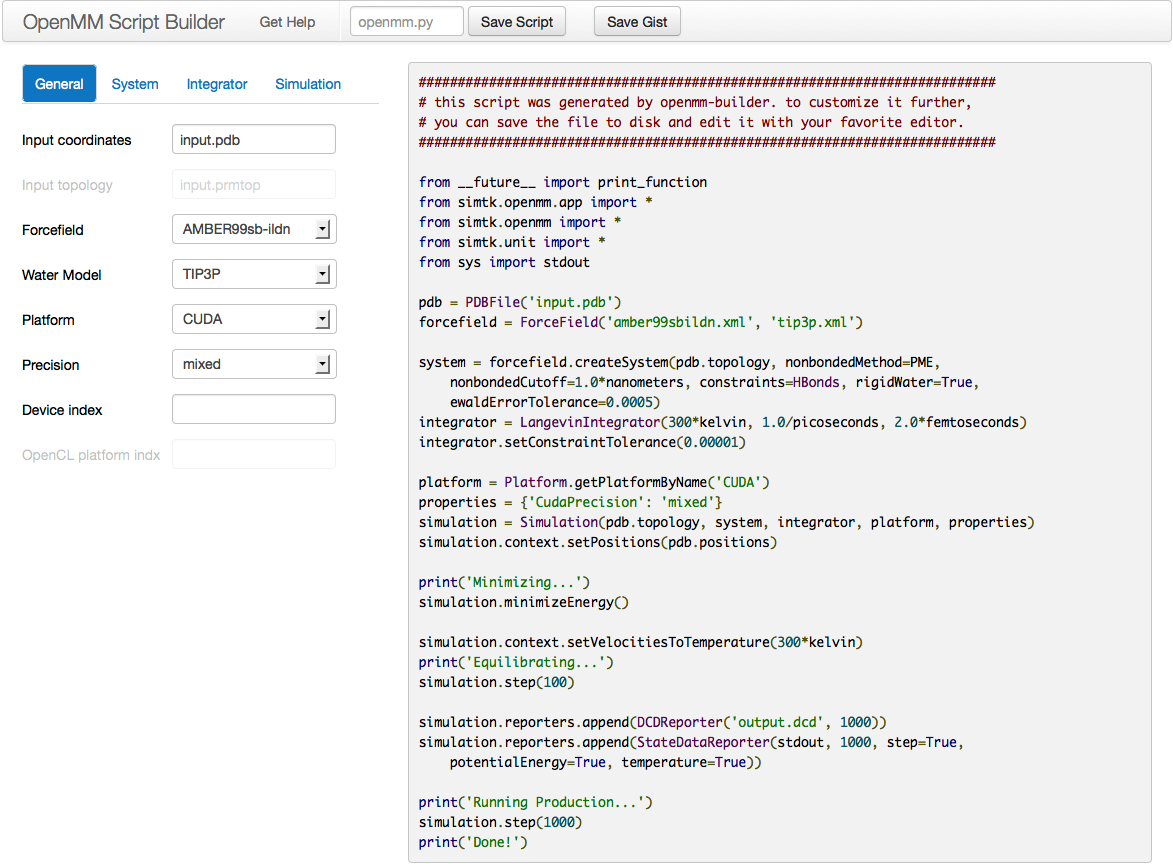
Figure 4-1: The Script Builder application

This is a web application available at https://builder.openmm.org. It provides a graphical interface with simple choices for all the most common simulation options, then automatically generates a script based on them. As you change the settings, the script is instantly updated to reflect them. Once everything is set the way you want, click the Save Script button to save it to disk, or simply copy and paste it into a text editor.

4.6. Simulation Parameters¶

Now let’s consider lots of ways you might want to customize your script.

4.6.1. Platforms¶

When creating a Simulation, you can optionally tell it what Platform to use. OpenMM includes four platforms: Reference, CPU, CUDA, and OpenCL. For a description of the differences between them, see Section 8.7. If you do not specify a Platform, it will select one automatically. Usually its choice will be reasonable, but you may want to change it.

The following lines specify to use the CUDA platform:

platform = Platform.getPlatformByName('CUDA')
simulation = Simulation(prmtop.topology, system, integrator, platform)

The platform name should be one of OpenCL, CUDA, CPU, or Reference.

You also can specify platform-specific properties that customize how calculations should be done. See Chapter 11 for details of the properties that each Platform supports. For example, the following lines specify to parallelize work across two different GPUs (CUDA devices 0 and 1), doing all computations in double precision:

platform = Platform.getPlatformByName('CUDA')
properties = {'CudaDeviceIndex': '0,1', 'CudaPrecision': 'double'}
simulation = Simulation(prmtop.topology, system, integrator, platform, properties)

4.6.2. Force Fields¶

When you create a force field, you specify one or more XML files from which to load the force field definition. Most often, there will be one file to define the main force field, and possibly a second file to define the water model (either implicit or explicit). For example:

forcefield = ForceField('amber99sb.xml', 'tip3p.xml')

For the main force field, OpenMM provides the following options:

File	Force Field
amber96.xml	Amber96[1]
amber99sb.xml	Amber99[2] with modified backbone torsions[3]
amber99sbildn.xml	Amber99SB plus improved side chain torsions[4]
amber99sbnmr.xml	Amber99SB with modifications to fit NMR data[5]
amber03.xml	Amber03[6]
amber10.xml	Amber10 (documented in the AmberTools manual as ff10)
amoeba2009.xml	AMOEBA 2009[7]. This force field is deprecated. It is recommended to use AMOEBA 2013 instead.
amoeba2013.xml	AMOEBA 2013[8]
charmm_polar_2013.xml	CHARMM 2013 polarizable force field[9]

The AMBER files do not include parameters for water molecules. This allows you to separately select which water model you want to use. For simulations that include explicit water molecules, you should also specify one of the following files:

File	Water Model
tip3p.xml	TIP3P water model[10]
tip3pfb.xml	TIP3P-FB water model[11]
tip4pew.xml	TIP4P-Ew water model[12]
tip4pfb.xml	TIP4P-FB water model[11]
tip5p.xml	TIP5P water model[13]
spce.xml	SPC/E water model[14]
swm4ndp.xml	SWM4-NDP water model[15]

For the polarizable force fields (AMOEBA and CHARMM), only one explicit water model is currently available and the water parameters are included in the same file as the macromolecule parameters. Also, the polarizable force fields only include parameters for amino acids and ions, not for nucleic acids.

If you want to include an implicit solvation model, you can also specify one of the following files:

File	Implicit Solvation Model
amber96_obc.xml	GBSA-OBC solvation model[16] for use with Amber96 force field
amber99_obc.xml	GBSA-OBC solvation model for use with Amber99 force fields
amber03_obc.xml	GBSA-OBC solvation model for use with Amber03 force field
amber10_obc.xml	GBSA-OBC solvation model for use with Amber10 force field
amoeba2009_gk.xml	Generalized Kirkwood solvation model[17] for use with AMOEBA 2009 force field
amoeba2013_gk.xml	Generalized Kirkwood solvation model for use with AMOEBA 2013 force field

For example, to use the GBSA-OBC solvation model with the Amber99SB force field, you would type:

forcefield = ForceField('amber99sb.xml', 'amber99_obc.xml')

Note that the GBSA-OBC parameters in these files are those used in TINKER.[18] They are designed for use with Amber force fields, but they are different from the parameters found in the AMBER application.

If you are running a vacuum simulation, you do not need to specify a water model. The following line specifies the Amber10 force field and no water model. If you try to use it with a PDB file that contains explicit water, it will produce an error since no water parameters are defined:

forcefield = ForceField('amber10.xml')

Be aware that some force fields and water models include “extra particles”, such as lone pairs or Drude particles. Examples include the CHARMM polarizable force field and all of the 4 and 5 site water models. To use these force fields, you must first add the extra particles to the Topology. See section 5.3 for details.

4.6.3. AMBER Implicit Solvent¶

When creating a system from a prmtop file you do not specify force field files, so you need a different way to tell it to use implicit solvent. This is done with the implicitSolvent parameter:

system = prmtop.createSystem(implicitSolvent=OBC2)

OpenMM supports all of the Generalized Born models used by AMBER. Here are the allowed values for implicitSolvent:

Value	Meaning
None	No implicit solvent is used.
HCT	Hawkins-Cramer-Truhlar GBSA model[19] (corresponds to igb=1 in AMBER)
OBC1	Onufriev-Bashford-Case GBSA model[16] using the GB^OBCI parameters (corresponds to igb=2 in AMBER).
OBC2	Onufriev-Bashford-Case GBSA model[16] using the GB^OBCII parameters (corresponds to igb=5 in AMBER). This is the same model used by the GBSA-OBC files described in Section 4.6.2.
GBn	GBn solvation model[20] (corresponds to igb=7 in AMBER).
GBn2	GBn2 solvation model[21] (corresponds to igb=8 in AMBER).

You can further control the solvation model in a few ways. First, you can specify the dielectric constants to use for the solute and solvent:

system = prmtop.createSystem(implicitSolvent=OBC2, soluteDielectric=1.0,
        solventDielectric=80.0)

If they are not specified, the solute and solvent dielectrics default to 1.0 and 78.5, respectively. These values were chosen for consistency with AMBER, and are slightly different from those used elsewhere in OpenMM: when building a system from a force field, the solvent dielectric defaults to 78.3.

You also can model the effect of a non-zero salt concentration by specifying the Debye-Huckel screening parameter[22]:

system = prmtop.createSystem(implicitSolvent=OBC2, implicitSolventKappa=1.0/nanometer)

4.6.4. Nonbonded Interactions¶

When creating the system (either from a force field or a prmtop file), you can specify options about how nonbonded interactions should be treated:

system = prmtop.createSystem(nonbondedMethod=PME, nonbondedCutoff=1*nanometer)

The nonbondedMethod parameter can have any of the following values:

Value	Meaning
NoCutoff	No cutoff is applied.
CutoffNonPeriodic	The reaction field method is used to eliminate all interactions beyond a cutoff distance. Not valid for AMOEBA.
CutoffPeriodic	The reaction field method is used to eliminate all interactions beyond a cutoff distance. Periodic boundary conditions are applied, so each atom interacts only with the nearest periodic copy of every other atom. Not valid for AMOEBA.
Ewald	Periodic boundary conditions are applied. Ewald summation is used to compute long range interactions. (This option is rarely used, since PME is much faster for all but the smallest systems.) Not valid for AMOEBA.
PME	Periodic boundary conditions are applied. The Particle Mesh Ewald method is used to compute long range interactions.

When using any method other than NoCutoff, you should also specify a cutoff distance. Be sure to specify units, as shown in the examples above. For example, nonbondedCutoff=1.5*nanometers or nonbondedCutoff=12*angstroms are legal values.

When using Ewald or PME, you can optionally specify an error tolerance for the force computation. For example:

system = prmtop.createSystem(nonbondedMethod=PME, nonbondedCutoff=1*nanometer,
        ewaldErrorTolerance=0.00001)

The error tolerance is roughly equal to the fractional error in the forces due to truncating the Ewald summation. If you do not specify it, a default value of 0.0005 is used.

4.6.4.1. Nonbonded Forces for AMOEBA¶

For the AMOEBA force field, the valid values for the nonbondedMethod are NoCutoff and PME. The other nonbonded methods, CutoffNonPeriodic, CutoffPeriodic, and Ewald are unavailable for this force field.

For implicit solvent runs using AMOEBA, only the nonbondedMethod option NoCutoff is available.

4.6.4.1.1. Lennard-Jones Interaction Cutoff Value¶

In addition, for the AMOEBA force field a cutoff for the Lennard-Jones interaction independent of the value used for the electrostatic interactions may be specified using the keyword vdwCutoff.

system = forcefield.createSystem(nonbondedMethod=PME, nonbondedCutoff=1*nanometer,
        ewaldErrorTolerance=0.00001, vdwCutoff=1.2*nanometer)

If vdwCutoff is not specified, then the value of nonbondedCutoff is used for the Lennard-Jones interactions.

4.6.4.1.2. Specifying the Polarization Method¶

OpenMM allows the setting of several other parameters particular to the AMOEBA force field. The mutualInducedTargetEpsilon option allows you to specify the accuracy to which the induced dipoles are calculated at each time step; the default value is 0.01. The polarization setting determines whether the calculation of the induced dipoles is continued until the dipoles are self-consistent to within the tolerance specified by mutualInducedTargetEpsilon or whether a quick estimate of the induced dipoles is used instead. The first option corresponds to the polarization=’mutual’ setting and is the default; the quick estimate option is given by polarization=’direct’ and in this case, mutualInducedTargetEpsilon is ignored, if provided. Simulations using polarization=’direct’ will be significantly faster than those with polarization=’mutual’, but less accurate. Examples using the two options are given below:

system = forcefield.createSystem(nonbondedMethod=PME,
    nonbondedCutoff=1*nanometer,ewaldErrorTolerance=0.00001,
    vdwCutoff=1.2*nanometer, mutualInducedTargetEpsilon=0.01)

system = forcefield.createSystem(nonbondedMethod=PME,
    nonbondedCutoff=1*nanometer,ewaldErrorTolerance=0.00001,
    vdwCutoff=1.2*nanometer, polarization ='direct')

4.6.4.1.3. Implicit Solvent and Solute Dielectrics¶

For implicit solvent simulations using the AMOEBA force field, the amoeba2013_gk.xml file should be included in the initialization of the force field:

forcefield = ForceField('amoeba2009.xml', 'amoeba2009_gk.xml')

Only the nonbondedMethod option NoCutoff is available for implicit solvent runs using AMOEBA. In addition, the solvent and solute dielectric values can be specified for implicit solvent simulations:

system=forcefield.createSystem(nonbondedMethod=NoCutoff, soluteDielectric=2.0,
        solventDielectric=80.0)

The default values are 1.0 for the solute dielectric and 78.3 for the solvent dielectric.

4.6.5. Constraints¶

When creating the system (either from a force field or an AMBER prmtop file), you can optionally tell OpenMM to constrain certain bond lengths and angles. For example,

system = prmtop.createSystem(nonbondedMethod=NoCutoff, constraints=HBonds)

The constraints parameter can have any of the following values:

Value	Meaning
None	No constraints are applied. This is the default value.
HBonds	The lengths of all bonds that involve a hydrogen atom are constrained.
AllBonds	The lengths of all bonds are constrained.
HAngles	The lengths of all bonds are constrained. In addition, all angles of the form H-X-H or H-O-X (where X is an arbitrary atom) are constrained.

The main reason to use constraints is that it allows one to use a larger integration time step. With no constraints, one is typically limited to a time step of about 1 fs for typical biomolecular force fields like AMBER or CHARMM. With HBonds constraints, this can be increased to about 2 fs. With HAngles, it can be further increased to 3.5 or 4 fs.

Regardless of the value of this parameter, OpenMM makes water molecules completely rigid, constraining both their bond lengths and angles. You can disable this behavior with the rigidWater parameter:

system = prmtop.createSystem(nonbondedMethod=NoCutoff, constraints=None, rigidWater=False)

Be aware that flexible water may require you to further reduce the integration step size, typically to about 0.5 fs.

Note

The AMOEBA forcefield is intended to be used without constraints.

4.6.6. Heavy Hydrogens¶

When creating the system (either from a force field or an AMBER prmtop file), you can optionally tell OpenMM to increase the mass of hydrogen atoms. For example,

system = prmtop.createSystem(hydrogenMass=4*amu)

This applies only to hydrogens that are bonded to heavy atoms, and any mass added to the hydrogen is subtracted from the heavy atom. This keeps their total mass constant while slowing down the fast motions of hydrogens. When combined with constraints (typically constraints=AllBonds), this allows a further increase in integration step size.

4.6.7. Integrators¶

OpenMM offers a choice of several different integration methods. You select which one to use by creating an integrator object of the appropriate type.

4.6.7.1. Langevin Integrator¶

In the examples of the previous sections, we used Langevin integration:

integrator = LangevinIntegrator(300*kelvin, 1/picosecond, 0.002*picoseconds)

The three parameter values in this line are the simulation temperature (300 K), the friction coefficient (1 ps^-1), and the step size (0.002 ps). You are free to change these to whatever values you want. Be sure to specify units on all values. For example, the step size could be written either as 0.002*picoseconds or 2*femtoseconds. They are exactly equivalent.

4.6.7.2. Leapfrog Verlet Integrator¶

A leapfrog Verlet integrator can be used for running constant energy dynamics. The command for this is:

integrator = VerletIntegrator(0.002*picoseconds)

The only option is the step size.

4.6.7.3. Brownian Integrator¶

Brownian (diffusive) dynamics can be used by specifying the following:

integrator = BrownianIntegrator(300*kelvin, 1/picosecond, 0.002*picoseconds)

The parameters are the same as for Langevin dynamics: temperature (300 K), friction coefficient (1 ps^-1), and step size (0.002 ps).

4.6.7.4. Variable Time Step Langevin Integrator¶

A variable time step Langevin integrator continuously adjusts its step size to keep the integration error below a specified tolerance. In some cases, this can allow you to use a larger average step size than would be possible with a fixed step size integrator. It also is very useful in cases where you do not know in advance what step size will be stable, such as when first equilibrating a system. You create this integrator with the following command:

integrator = VariableLangevinIntegrator(300*kelvin, 1/picosecond, 0.001)

In place of a step size, you specify an integration error tolerance (0.001 in this example). It is best not to think of this value as having any absolute meaning. Just think of it as an adjustable parameter that affects the step size and integration accuracy. Smaller values will produce a smaller average step size. You should try different values to find the largest one that produces a trajectory sufficiently accurate for your purposes.

4.6.7.5. Variable Time Step Leapfrog Verlet Integrator¶

A variable time step leapfrog Verlet integrator works similarly to the variable time step Langevin integrator in that it continuously adjusts its step size to keep the integration error below a specified tolerance. The command for this integrator is:

integrator = VariableVerletIntegrator(0.001)

The parameter is the integration error tolerance (0.001), whose meaning is the same as for the Langevin integrator.

4.6.7.6. Multiple Time Step Integrator¶

The MTSIntegrator class implements the rRESPA multiple time step algorithm[23]. This allows some forces in the system to be evaluated more frequently than others. For details on how to use it, consult the API documentation.

4.6.7.7. aMD Integrator¶

There are three different integrator types that implement variations of the aMD[24] accelerated sampling algorithm: AMDIntegrator, AMDForceGroupIntegrator, and DualAMDIntegrator. They perform integration on a modified potential energy surface to allow much faster sampling of conformations. For details on how to use them, consult the API documentation.

4.6.8. Temperature Coupling¶

If you want to run a simulation at constant temperature, using a Langevin integrator (as shown in the examples above) is usually the best way to do it. OpenMM does provide an alternative, however: you can use a Verlet integrator, then add an Andersen thermostat to your system to provide temperature coupling.

To do this, we can add an AndersenThermostat object to the System as shown below.

...
system = prmtop.createSystem(nonbondedMethod=PME, nonbondedCutoff=1*nanometer,
        constraints=HBonds)
system.addForce(AndersenThermostat(300*kelvin, 1/picosecond))
integrator = VerletIntegrator(0.002*picoseconds)
...

The two parameters of the Andersen thermostat are the temperature (300 K) and collision frequency (1 ps^-1).

4.6.9. Pressure Coupling¶

All the examples so far have been constant volume simulations. If you want to run at constant pressure instead, add a Monte Carlo barostat to your system. You do this exactly the same way you added the Andersen thermostat in the previous section:

...
system = prmtop.createSystem(nonbondedMethod=PME, nonbondedCutoff=1*nanometer,
        constraints=HBonds)
system.addForce(MonteCarloBarostat(1*bar, 300*kelvin))
integrator = LangevinIntegrator(300*kelvin, 1/picosecond, 0.002*picoseconds)
...

The parameters of the Monte Carlo barostat are the pressure (1 bar) and temperature (300 K). The barostat assumes the simulation is being run at constant temperature, but it does not itself do anything to regulate the temperature.

Warning

It is therefore critical that you always use it along with a Langevin integrator or Andersen thermostat, and that you specify the same temperature for both the barostat and the integrator or thermostat. Otherwise, you will get incorrect results.

There also is an anisotropic barostat that scales each axis of the periodic box independently, allowing it to change shape. When using the anisotropic barostat, you can specify a different pressure for each axis. The following line applies a pressure of 1 bar along the X and Y axes, but a pressure of 2 bar along the Z axis:

system.addForce(MonteCarloAnisotropicBarostat((1, 1, 2)*bar, 300*kelvin))

Another feature of the anisotropic barostat is that it can be applied to only certain axes of the periodic box, keeping the size of the other axes fixed. This is done by passing three additional parameters that specify whether the barostat should be applied to each axis. The following line specifies that the X and Z axes of the periodic box should not be scaled, so only the Y axis can change size.

system.addForce(MonteCarloAnisotropicBarostat((1, 1, 1)*bar, 300*kelvin,
        False, True, False))

There is a third barostat designed specifically for simulations of membranes. It assumes the membrane lies in the XY plane, and treats the X and Y axes of the box differently from the Z axis. It also applies a uniform surface tension in the plane of the membrane. The following line adds a membrane barostat that applies a pressure of 1 bar and a surface tension of 200 bar*nm. It specifies that the X and Y axes are treated isotropically while the Z axis is free to change independently.

system.addForce(MonteCarloMembraneBarostat(1*bar, 200*bar*nanometer,
    MonteCarloMembraneBarostat.XYIsotropic, MonteCarloMembraneBarostat.ZFree, 300*kelvin))

See the API documentation for details about the allowed parameter values and their meanings.

4.6.10. Energy Minimization¶

As seen in the examples, performing a local energy minimization takes a single line in the script:

simulation.minimizeEnergy()

In most cases, that is all you need. There are two optional parameters you can specify if you want further control over the minimization. First, you can specify a tolerance for when the energy should be considered to have converged:

simulation.minimizeEnergy(tolerance=5*kilojoule/mole)

If you do not specify this parameter, a default tolerance of 10 kJ/mole is used.

Second, you can specify a maximum number of iterations:

simulation.minimizeEnergy(maxIterations=100)

The minimizer will exit once the specified number of iterations is reached, even if the energy has not yet converged. If you do not specify this parameter, the minimizer will continue until convergence is reached, no matter how many iterations it takes.

These options are independent. You can specify both if you want:

simulation.minimizeEnergy(tolerance=0.1*kilojoule/mole, maxIterations=500)

4.6.11. Removing Center of Mass Motion¶

By default, System objects created with the OpenMM application tools add a CMMotionRemover that removes all center of mass motion at every time step so the system as a whole does not drift with time. This is almost always what you want. In rare situations, you may want to allow the system to drift with time. You can do this by specifying the removeCMMotion parameter when you create the System:

system = forcefield.createSystem(pdb.topology, nonbondedMethod=NoCutoff,
        removeCMMotion=False)

4.6.12. Writing Trajectories¶

OpenMM can save simulation trajectories to disk in two formats: PDB and DCD. Both of these are widely supported formats, so you should be able to read them into most analysis and visualization programs.

To save a trajectory, just add a “reporter” to the simulation, as shown in the example scripts above:

simulation.reporters.append(PDBReporter('output.pdb', 1000))

The two parameters of the PDBReporter are the output filename and how often (in number of time steps) output structures should be written. To use DCD format, just replace PDBReporter with DCDReporter. The parameters represent the same values:

simulation.reporters.append(DCDReporter('output.dcd', 1000))

4.6.13. Recording Other Data¶

In addition to saving a trajectory, you may want to record other information over the course of a simulation, such as the potential energy or temperature. OpenMM provides a reporter for this purpose also. Create a StateDataReporter and add it to the simulation:

simulation.reporters.append(StateDataReporter('data.csv', 1000, time=True,
        kineticEnergy=True, potentialEnergy=True))

The first two parameters are the output filename and how often (in number of time steps) values should be written. The remaining arguments specify what values should be written at each report. The available options are step (the index of the current time step), time, progress (what percentage of the simulation has completed), remainingTime (an estimate of how long it will take the simulation to complete), potentialEnergy, kineticEnergy, totalEnergy, temperature, volume (the volume of the periodic box), density (the total system mass divided by the volume of the periodic box), and speed (an estimate of how quickly the simulation is running). If you include either the progress or remainingTime option, you must also include the totalSteps parameter to specify the total number of time steps that will be included in the simulation. One line is written to the file for each report containing the requested values. By default the values are written in comma-separated-value (CSV) format. You can use the separator parameter to choose a different separator. For example, the following line will cause values to be separated by spaces instead of commas:

simulation.reporters.append(StateDataReporter('data.txt', 1000, progress=True,
        temperature=True, totalSteps=10000, separator=' '))

5. Model Building and Editing¶

Sometimes you have a PDB file that needs some work before you can simulate it. Maybe it doesn’t contain hydrogen atoms (which is common for structures determined by X-ray crystallography), so you need to add them. Or perhaps you want to simulate the system in explicit water, but the PDB file doesn’t contain water molecules. Or maybe it does contain water molecules, but they contain the wrong number of interaction sites for the water model you want to use. OpenMM’s Modeller class can fix problems such as these.

To use it, create a Modeller object, providing the initial Topology and atom positions. You then can invoke various modelling functions on it. Each one modifies the system in some way, creating a new Topology and list of positions. When you are all done, you can retrieve them from the Modeller and use them as the starting point for your simulation:

...
pdb = PDBFile('input.pdb')
modeller = Modeller(pdb.topology, pdb.positions)
# ... Call some modelling functions here ...
system = forcefield.createSystem(modeller.topology, nonbondedMethod=PME)
simulation = Simulation(modeller.topology, system, integrator)
simulation.context.setPositions(modeller.positions)

Example 5-1

Now let’s consider the particular functions you can call.

5.1. Adding Hydrogens¶

Call the addHydrogens() function to add missing hydrogen atoms:

modeller.addHydrogens(forcefield)

The force field is needed to determine the positions for the hydrogen atoms. If the system already contains some hydrogens but is missing others, that is fine. The Modeller will recognize the existing ones and figure out which ones need to be added.

Some residues can exist in different protonation states depending on the pH and on details of the local environment. By default it assumes pH 7, but you can specify a different value:

modeller.addHydrogens(forcefield, pH=5.0)

For each residue, it selects the protonation state that is most common at the specified pH. In the case of Cysteine residues, it also checks whether the residue participates in a disulfide bond when selecting the state to use. Histidine has two different protonation states that are equally likely at neutral pH. It therefore selects which one to use based on which will form a better hydrogen bond.

If you want more control, it is possible to specify exactly which protonation state to use for particular residues. For details, consult the API documentation for the Modeller class.

5.2. Adding Solvent¶

Call addSolvent() to create a box of solvent (water and ions) around the model:

modeller.addSolvent(forcefield)

This constructs a box of water around the solute, ensuring that no water molecule comes closer to any solute atom than the sum of their van der Waals radii. It also determines the charge of the solute, and adds enough positive or negative ions to make the system neutral.

When called as shown above, addSolvent() expects that periodic box dimensions were specified in the PDB file, and it uses them as the size for the water box. If your PDB file does not specify a box size, or if you want to use a different size, you can specify one:

modeller.addSolvent(forcefield, boxSize=Vec3(5.0, 3.5, 3.5)*nanometers)

This requests a 5 nm by 3.5 nm by 3.5 nm box. For a non-rectangular box, you can specify the three box vectors defining the unit cell:

modeller.addSolvent(forcefield, boxVectors=(avec, bvec, cvec))

Another option is to specify a padding distance:

modeller.addSolvent(forcefield, padding=1.0*nanometers)

This determines the largest size of the solute along any axis (x, y, or z). It then creates a cubic box of width (solute size)+2*(padding). The above line guarantees that no part of the solute comes closer than 1 nm to any edge of the box.

Finally, you can specify the exact number of solvent molecules (including both water and ions) to add. This is useful when you want to solvate several different conformations of the same molecule while guaranteeing they all have the same amount of solvent:

modeller.addSolvent(forcefield, numAdded=5000)

By default, addSolvent() creates TIP3P water molecules, but it also supports other water models:

modeller.addSolvent(forcefield, model='tip5p')

Allowed values for the model option are 'tip3p', 'tip3pfb', 'spce', 'tip4pew', 'tip4pfb', and 'tip5p'. Be sure to include the single quotes around the value.

Another option is to add extra ion pairs to give a desired total ionic strength. For example:

modeller.addSolvent(forcefield, ionicStrength=0.1*molar)

This solvates the system with a salt solution whose ionic strength is 0.1 molar. Note that when computing the ionic strength, it does not consider the ions that were added to neutralize the solute. It assumes those are bound to the solute and do not contribute to the bulk ionic strength.

By default, Na⁺ and Cl^- ions are used, but you can specify different ones using the positiveIon and negativeIon options. For example, this creates a potassium chloride solution:

modeller.addSolvent(forcefield, ionicStrength=0.1*molar, positiveIon='K+')

Allowed values for positiveIon are 'Cs+', 'K+', 'Li+', 'Na+', and 'Rb+'. Allowed values for negativeIon are 'Cl-', 'Br-', 'F-', and 'I-'. Be sure to include the single quotes around the value. Also be aware some force fields do not include parameters for all of these ion types, so you need to use types that are supported by your chosen force field.

5.3. Adding or Removing Extra Particles¶

“Extra particles” are particles that do not represent ordinary atoms. This includes the virtual interaction sites used in many water models, Drude particles, etc. If you are using a force field that involves extra particles, you must add them to the Topology. To do this, call:

modeller.addExtraParticles(forcefield)

This looks at the force field to determine what extra particles are needed, then modifies each residue to include them. This function can remove extra particles as well as adding them.

5.4. Removing Water¶

Call deleteWater to remove all water molecules from the system:

modeller.deleteWater()

This is useful, for example, if you want to simulate it with implicit solvent. Be aware, though, that this only removes water molecules, not ions or other small molecules that might be considered “solvent”.

5.5. Saving The Results¶

Once you have finished editing your model, you can immediately use the resulting Topology object and atom positions as the input to a Simulation. If you plan to simulate it many times, though, it is usually better to save the result to a new PDB file, then use that as the input for the simulations. This avoids the cost of repeating the modelling operations at the start of every simulation, and also ensures that all your simulations are really starting from exactly the same structure.

The following example loads a PDB file, adds missing hydrogens, builds a solvent box around it, performs an energy minimization, and saves the result to a new PDB file.

from simtk.openmm.app import *
from simtk.openmm import *
from simtk.unit import *

print('Loading...')
pdb = PDBFile('input.pdb')
forcefield = ForceField('amber99sb.xml', 'tip3p.xml')
modeller = Modeller(pdb.topology, pdb.positions)
print('Adding hydrogens...')
modeller.addHydrogens(forcefield)
print('Adding solvent...')
modeller.addSolvent(forcefield, model='tip3p', padding=1*nanometer)
print('Minimizing...')
system = forcefield.createSystem(modeller.topology, nonbondedMethod=PME)
integrator = VerletIntegrator(0.001*picoseconds)
simulation = Simulation(modeller.topology, system, integrator)
simulation.context.setPositions(modeller.positions)
simulation.minimizeEnergy(maxIterations=100)
print('Saving...')
positions = simulation.context.getState(getPositions=True).getPositions()
PDBFile.writeFile(simulation.topology, positions, open('output.pdb', 'w'))
print('Done')

Example 5-2

6. Advanced Simulation Examples¶

In the previous chapter, we looked at some basic scripts for running simulations and saw lots of ways to customize them. If that is all you want to do—run straightforward molecular simulations—you already know everything you need to know. Just use the example scripts and customize them in the ways described in Section 4.6.

OpenMM can do far more than that. Your script has the full OpenMM API at its disposal, along with all the power of the Python language and libraries. In this chapter, we will consider some examples that illustrate more advanced techniques. Remember that these are still only examples; it would be impossible to give an exhaustive list of everything OpenMM can do. Hopefully they will give you a sense of what is possible, and inspire you to experiment further on your own.

Starting in this section, we will assume some knowledge of programming, as well as familiarity with the OpenMM API. Consult the OpenMM Users Guide and API documentation if you are uncertain about how something works. You can also use the Python help command. For example,

help(Simulation)

will print detailed documentation on the Simulation class.

6.1. Simulated Annealing¶

Here is a very simple example of how to do simulated annealing. The following lines linearly reduce the temperature from 300 K to 0 K in 100 increments, executing 1000 time steps at each temperature:

...
simulation.context.setPositions(pdb.positions)
simulation.minimizeEnergy()
for i in range(100):
    integrator.setTemperature(3*(100-i)*kelvin)
    simulation.step(1000)

Example 6-1

This code needs very little explanation. The loop is executed 100 times. Each time through, it adjusts the temperature of the LangevinIntegrator and then calls step(1000) to take 1000 time steps.

6.2. Applying an External Force to Particles: a Spherical Container¶

In this example, we will simulate a non-periodic system contained inside a spherical container with radius 2 nm. We implement the container by applying a harmonic potential to every particle:

\[\begin{split}E(r) = \begin{cases} 0 & r\le2\\ 100(r-2)^2 & r>2 \end{cases}\end{split}\]

where r is the distance of the particle from the origin, measured in nm. We can easily do this using OpenMM’s CustomExternalForce class. This class applies a force to some or all of the particles in the system, where the energy is an arbitrary function of each particle’s (x, y, z) coordinates. Here is the code to do it:

...
system = forcefield.createSystem(pdb.topology, nonbondedMethod=CutoffNonPeriodic,
        nonbondedCutoff=1*nanometer, constraints=None)
force = CustomExternalForce('100*max(0, r-2)^2; r=sqrt(x*x+y*y+z*z)')
system.addForce(force)
for i in range(system.getNumParticles()):
    force.addParticle(i, [])
integrator = LangevinIntegrator(300*kelvin, 91/picosecond, 0.002*picoseconds)
...

Example 6-2

The first thing it does is create a CustomExternalForce object and add it to the System. The argument to CustomExternalForce is a mathematical expression specifying the potential energy of each particle. This can be any function of x, y, and z you want. It also can depend on global or per-particle parameters. A wide variety of restraints, steering forces, shearing forces, etc. can be implemented with this method.

Next it must specify which particles to apply the force to. In this case, we want it to affect every particle in the system, so we loop over them and call addParticle() once for each one. The two arguments are the index of the particle to affect, and the list of per-particle parameter values (an empty list in this case). If we had per-particle parameters, such as to make the force stronger for some particles than for others, this is where we would specify them.

Notice that we do all of this immediately after creating the System. That is not an arbitrary choice.

Warning

If you add new forces to a System, you must do so before creating the Simulation. Once you create a Simulation, modifying the System will have no effect on that Simulation.

6.3. Extracting and Reporting Forces (and other data)¶

OpenMM provides reporters for two output formats: PDB and DCD. Both of those formats store only positions, not velocities, forces, or other data. In this section, we create a new reporter that outputs forces. This illustrates two important things: how to write a reporter, and how to query the simulation for forces or other data.

Here is the definition of the ForceReporter class:

class ForceReporter(object):
    def __init__(self, file, reportInterval):
        self._out = open(file, 'w')
        self._reportInterval = reportInterval

    def __del__(self):
        self._out.close()

    def describeNextReport(self, simulation):
        steps = self._reportInterval - simulation.currentStep%self._reportInterval
        return (steps, False, False, True, False)

    def report(self, simulation, state):
        forces = state.getForces().value_in_unit(kilojoules/mole/nanometer)
        for f in forces:
            self._out.write('%g %g %g\n' % (f[0], f[1], f[2]))

Example 6-3

The constructor and destructor are straightforward. The arguments to the constructor are the output filename and the interval (in time steps) at which it should generate reports. It opens the output file for writing and records the reporting interval. The destructor closes the file.

We then have two methods that every reporter must implement: describeNextReport() and report(). A Simulation object periodically calls describeNextReport() on each of its reporters to find out when that reporter will next generate a report, and what information will be needed to generate it. The return value should be a five element tuple, whose elements are as follows:

The number of time steps until the next report. We calculate this as (report interval)-(current step)%(report interval). For example, if we want a report every 100 steps and the simulation is currently on step 530, we will return 100-(530%100) = 70.
Whether the next report will need particle positions.
Whether the next report will need particle velocities.
Whether the next report will need forces.
Whether the next report will need energies.

When the time comes for the next scheduled report, the Simulation calls report() to generate the report. The arguments are the Simulation object, and a State that is guaranteed to contain all the information that was requested by describeNextReport(). A State object contains a snapshot of information about the simulation, such as forces or particle positions. We call getForces() to retrieve the forces and convert them to the units we want to output (kJ/mole/nm). Then we loop over each value and write it to the file. To keep the example simple, we just print the values in text format, one line per particle. In a real program, you might choose a different output format.

Now that we have defined this class, we can use it exactly like any other reporter. For example,

simulation.reporters.append(ForceReporter('forces.txt', 100))

will output forces to a file called “forces.txt” every 100 time steps.

6.4. Computing Energies¶

This example illustrates a different sort of analysis. Instead of running a simulation, assume we have already identified a set of structures we are interested in. These structures are saved in a set of PDB files. We want to loop over all the files in a directory, load them in one at a time, and compute the potential energy of each one. Assume we have already created our System and Simulation. The following lines perform the analysis:

import os
for file in os.listdir('structures'):
    pdb = PDBFile(os.path.join('structures', file))
    simulation.context.setPositions(pdb.positions)
    state = simulation.context.getState(getEnergy=True)
    print file, state.getPotentialEnergy()

Example 6-4

We use Python’s listdir() function to list all the files in the directory. We create a PDBFile object for each one and call setPositions() on the Context to specify the particle positions loaded from the PDB file. We then compute the energy by calling getState() with the option getEnergy=True, and print it to the console along with the name of the file.

7. Creating Force Fields¶

OpenMM uses a simple XML file format to describe force fields. It includes many common force fields, but you can also create your own. A force field can use all the standard OpenMM force classes, as well as the very flexible custom force classes. You can even extend the ForceField class to add support for completely new forces, such as ones defined in plugins. This makes it a powerful tool for force field development.

7.1. Basic Concepts¶

Let’s start by considering how OpenMM defines a force field. There are a small number of basic concepts to understand.

7.1.1. Atom Types and Atom Classes¶

Force field parameters are assigned to atoms based on their “atom types”. Atom types should be the most specific identification of an atom that will ever be needed. Two atoms should have the same type only if the force field will always treat them identically in every way.

Multiple atom types can be grouped together into “atom classes”. In general, two types should be in the same class if the force field usually (but not necessarily always) treats them identically. For example, the \(\alpha\)-carbon of an alanine residue will probably have a different atom type than the \(\alpha\)-carbon of a leucine residue, but both of them will probably have the same atom class.

All force field parameters can be specified either by atom type or atom class. Classes exist as a convenience to make force field definitions more compact. If necessary, you could define everything in terms of atom types, but when many types all share the same parameters, it is convenient to only have to specify them once.

7.1.2. Residue Templates¶

Types are assigned to atoms by matching residues to templates. A template specifies a list of atoms, the type of each one, and the bonds between them. For each residue in the PDB file, the force field searches its list of templates for one that has an identical set of atoms with identical bonds between them. When matching templates, neither the order of the atoms nor their names matter; it only cares about their elements and the set of bonds between them. (The PDB file reader does care about names, of course, since it needs to figure out which atom each line of the file corresponds to.)

7.1.3. Forces¶

Once a force field has defined its atom types and residue templates, it must define its force field parameters. This generally involves one block of XML for each Force object that will be added to the System. The details are different for each Force, but it generally consists of a set of rules for adding interactions based on bonds and atom types or classes. For example, when adding a HarmonicBondForce, the force field will loop over every pair of bonded atoms, check their types and classes, and see if they match any of its rules. If so, it will call addBond() on the HarmonicBondForce. If none of them match, it simply ignores that pair and continues.

7.2. Writing the XML File¶

The root element of the XML file must be a <ForceField> tag:

<ForceField>
...
</ForceField>

The <ForceField> tag contains the following children:

An <AtomTypes> tag containing the atom type definitions
A <Residues> tag containing the residue template definitions
Zero or more tags defining specific forces

The order of these tags does not matter. They are described in details below.

7.2.1. <AtomTypes>¶

The atom type definitions look like this:

<AtomTypes>
 <Type name="0" class="N" element="N" mass="14.00672"/>
 <Type name="1" class="H" element="H" mass="1.007947"/>
 <Type name="2" class="CT" element="C" mass="12.01078"/>
 ...
</AtomTypes>

There is one <Type> tag for each atom type. It specifies the name of the type, the name of the class it belongs to, the symbol for its element, and its mass in amu. The names are arbitrary strings: they need not be numbers, as in this example. The only requirement is that all types have unique names. The classes are also arbitrary strings, and in general will not be unique. Two types belong to the same class if they list the same value for the class attribute.

7.2.2. <Residues>¶

The residue template definitions look like this:

<Residues>
 <Residue name="ACE">
  <Atom name="HH31" type="710"/>
  <Atom name="CH3" type="711"/>
  <Atom name="HH32" type="710"/>
  <Atom name="HH33" type="710"/>
  <Atom name="C" type="712"/>
  <Atom name="O" type="713"/>
  <Bond from="0" to="1"/>
  <Bond from="1" to="2"/>
  <Bond from="1" to="3"/>
  <Bond from="1" to="4"/>
  <Bond from="4" to="5"/>
  <ExternalBond from="4"/>
 </Residue>
 <Residue name="ALA">
  ...
 </Residue>
 ...
</Residues>

There is one <Residue> tag for each residue template. That in turn contains the following tags:

An <Atom> tag for each atom in the residue. This specifies the name of the atom and its atom type.
A <Bond> tag for each pair of atoms that are bonded to each other. The to and from attributes are the indices of the two bonded atoms (starting from 0) in the order they were listed. For example, <Bond from=”1” to=”3”/> describes a bond between atom CH3 and atom HH33.
An <ExternalBond> tag for each atom that will be bonded to an atom of a different residue.

The <Residue> tag may also contain <VirtualSite> tags, as in the following example:

<Residue name="HOH">
 <Atom name="O" type="tip4pew-O"/>
 <Atom name="H1" type="tip4pew-H"/>
 <Atom name="H2" type="tip4pew-H"/>
 <Atom name="M" type="tip4pew-M"/>
 <VirtualSite type="average3" index="3" atom1="0" atom2="1" atom3="2"
     weight1="0.786646558" weight2="0.106676721" weight3="0.106676721"/>
 <Bond from="0" to="1"/>
 <Bond from="0" to="2"/>
</Residue>

Each <VirtualSite> tag indicates an atom in the residue that should be represented with a virtual site. The type attribute may equal “average2”, “average3”, or “outOfPlane”, which correspond to the TwoParticleAverageSite, ThreeParticleAverageSite, and OutOfPlaneSite classes respectively. The index attribute gives the index (starting from 0) of the atom to represent with a virtual site. The atoms it is calculated based on are specified by atom1, atom2, and (for virtual site classes that involve three atoms) atom3. The remaining attributes are specific to the virtual site class, and specify the parameters for calculating the site position. For a TwoParticleAverageSite, they are weight1 and weight2. For a ThreeParticleAverageSite, they are weight1, weight2, and weight3. For an OutOfPlaneSite, they are weight12, weight13, and weightCross.

7.2.3. <HarmonicBondForce>¶

To add a HarmonicBondForce to the System, include a tag that looks like this:

<HarmonicBondForce>
 <Bond class1="C" class2="C" length="0.1525" k="259408.0"/>
 <Bond class1="C" class2="CA" length="0.1409" k="392459.2"/>
 <Bond class1="C" class2="CB" length="0.1419" k="374049.6"/>
 ...
</HarmonicBondForce>

Every <Bond> tag defines a rule for creating harmonic bond interactions between atoms. Each tag may identify the atoms either by type (using the attributes type1 and type2) or by class (using the attributes class1 and class2). For every pair of bonded atoms, the force field searches for a rule whose atom types or atom classes match the two atoms. If it finds one, it calls addBond() on the HarmonicBondForce with the specified parameters. Otherwise, it ignores that pair and continues. length is the equilibrium bond length in nm, and k is the spring constant in kJ/mol/nm².

7.2.4. <HarmonicAngleForce>¶

To add a HarmonicAngleForce to the System, include a tag that looks like this:

<HarmonicAngleForce>
 <Angle class1="C" class2="C" class3="O" angle="2.094" k="669.44"/>
 <Angle class1="C" class2="C" class3="OH" angle="2.094" k="669.44"/>
 <Angle class1="CA" class2="C" class3="CA" angle="2.094" k="527.184"/>
 ...
</HarmonicAngleForce>

Every <Angle> tag defines a rule for creating harmonic angle interactions between triplets of atoms. Each tag may identify the atoms either by type (using the attributes type1, type2, ...) or by class (using the attributes class1, class2, ...). The force field identifies every set of three atoms in the system where the first is bonded to the second, and the second to the third. For each one, it searches for a rule whose atom types or atom classes match the three atoms. If it finds one, it calls addAngle() on the HarmonicAngleForce with the specified parameters. Otherwise, it ignores that set and continues. angle is the equilibrium angle in radians, and k is the spring constant in kJ/mol/radian².

7.2.5. <PeriodicTorsionForce>¶

To add a PeriodicTorsionForce to the System, include a tag that looks like this:

<PeriodicTorsionForce>
 <Proper class1="HC" class2="CT" class3="CT" class4="CT" periodicity1="3" phase1="0.0"
     k1="0.66944"/>
 <Proper class1="HC" class2="CT" class3="CT" class4="HC" periodicity1="3" phase1="0.0"
     k1="0.6276"/>
 ...
 <Improper class1="N" class2="C" class3="CT" class4="O" periodicity1="2"
     phase1="3.14159265359" k1="4.6024"/>
 <Improper class1="N" class2="C" class3="CT" class4="H" periodicity1="2"
     phase1="3.14159265359" k1="4.6024"/>
 ...
</PeriodicTorsionForce>

Every child tag defines a rule for creating periodic torsion interactions between sets of four atoms. Each tag may identify the atoms either by type (using the attributes type1, type2, ...) or by class (using the attributes class1, class2, ...).

The force field recognizes two different types of torsions: proper and improper. A proper torsion involves four atoms that are bonded in sequence: 1 to 2, 2 to 3, and 3 to 4. An improper torsion involves a central atom and three others that are bonded to it: atoms 2, 3, and 4 are all bonded to atom 1. The force field begins by identifying every set of atoms in the system of each of these types. For each one, it searches for a rule whose atom types or atom classes match the four atoms. If it finds one, it calls addTorsion() on the PeriodicTorsionForce with the specified parameters. Otherwise, it ignores that set and continues. periodicity1 is the periodicity of the torsion, phase1 is the phase offset in radians, and k1 is the force constant in kJ/mol.

Each torsion definition can specify multiple periodic torsion terms to add to its atoms. To add a second one, just add three more attributes: periodicity2, phase2, and k2. You can have as many terms as you want. Here is an example of a rule that adds three torsion terms to its atoms:

<Proper class1="CT" class2="CT" class3="CT" class4="CT"
    periodicity1="3" phase1="0.0" k1="0.75312"
    periodicity2="2" phase2="3.14159265359" k2="1.046"
    periodicity3="1" phase3="3.14159265359" k3="0.8368"/>

You can also use wildcards when defining torsions. To do this, simply leave the type or class name for an atom empty. That will cause it to match any atom. For example, the following definition will match any sequence of atoms where the second atom has class OS and the third has class P:

<Proper class1="" class2="OS" class3="P" class4="" periodicity1="3" phase1="0.0" k1="1.046"/>

7.2.6. <RBTorsionForce>¶

To add an RBTorsionForce to the System, include a tag that looks like this:

<RBTorsionForce>
 <Proper class1="CT" class2="CT" class3="OS" class4="CT" c0="2.439272" c1="4.807416"
     c2="-0.8368" c3="-6.409888" c4="0" c5="0" />
 <Proper class1="C" class2="N" class3="CT" class4="C" c0="10.46" c1="-3.34720"
     c2="-7.1128" c3="0" c4="0" c5="0" />
 ...
 <Improper class1="N" class2="C" class3="CT" class4="O" c0="0.8368" c1="0"
     c2="-2.76144" c3="0" c4="3.3472" c5="0" />
 <Improper class1="N" class2="C" class3="CT" class4="H" c0="29.288" c1="-8.368"
     c2="-20.92" c3="0" c4="0" c5="0" />
 ...
</RBTorsionForce>

Every child tag defines a rule for creating Ryckaert-Bellemans torsion interactions between sets of four atoms. Each tag may identify the atoms either by type (using the attributes type1, type2, ...) or by class (using the attributes class1, class2, ...).

The force field recognizes two different types of torsions: proper and improper. A proper torsion involves four atoms that are bonded in sequence: 1 to 2, 2 to 3, and 3 to 4. An improper torsion involves a central atom and three others that are bonded to it: atoms 2, 3, and 4 are all bonded to atom 1. The force field begins by identifying every set of atoms in the system of each of these types. For each one, it searches for a rule whose atom types or atom classes match the four atoms. If it finds one, it calls addTorsion() on the RBTorsionForce with the specified parameters. Otherwise, it ignores that set and continues. The attributes c0 through c5 are the coefficients of the terms in the Ryckaert-Bellemans force expression.

<Proper class1="" class2="OS" class3="P" class4="" c0="2.439272" c1="4.807416"
    c2="-0.8368" c3="-6.409888" c4="0" c5="0" />

7.2.7. <CMAPTorsionForce>¶

To add a CMAPTorsionForce to the System, include a tag that looks like this:

<CMAPTorsionForce>
 <Map>
  0.0 0.809 0.951 0.309
  -0.587 -1.0 -0.587 0.309
  0.951 0.809 0.0 -0.809
  -0.951 -0.309 0.587 1.0
 </Map>
 <Torsion map="0" class1="CT" class2="CT" class3="C" class4="N" class5="CT"/>
 <Torsion map="0" class1="N" class2="CT" class3="C" class4="N" class5="CT"/>
 ...
</CMAPTorsionForce>

Each <Map> tag defines an energy correction map. Its content is the list of energy values in kJ/mole, listed in the correct order for CMAPTorsionForce’s addMap() method and separated by white space. See the API documentation for details. The size of the map is determined from the number of energy values.

Each <Torsion> tag defines a rule for creating CMAP torsion interactions between sets of five atoms. The tag may identify the atoms either by type (using the attributes type1, type2, ...) or by class (using the attributes class1, class2, ...). The force field identifies every set of five atoms that are bonded in sequence: 1 to 2, 2 to 3, 3 to 4, and 4 to 5. For each one, it searches for a rule whose atom types or atom classes match the five atoms. If it finds one, it calls addTorsion() on the CMAPTorsionForce with the specified parameters. Otherwise, it ignores that set and continues. The first torsion is defined by the sequence of atoms 1-2-3-4, and the second one by atoms 2-3-4-5. map is the index of the map to use, starting from 0, in the order they are listed in the file.

You can also use wildcards when defining torsions. To do this, simply leave the type or class name for an atom empty. That will cause it to match any atom. For example, the following definition will match any sequence of five atoms where the middle three have classes CT, C, and N respectively:

<Torsion map="0" class1="" class2="CT" class3="C" class4="N" class5=""/>

7.2.8. <NonbondedForce>¶

To add a NonbondedForce to the System, include a tag that looks like this:

<NonbondedForce coulomb14scale="0.833333" lj14scale="0.5">
 <Atom type="0" charge="-0.4157" sigma="0.32499" epsilon="0.71128"/>
 <Atom type="1" charge="0.2719" sigma="0.10690" epsilon="0.06568"/>
 <Atom type="2" charge="0.0337" sigma="0.33996" epsilon="0.45772"/>
 ...
</NonbondedForce>

The <NonbondedForce> tag has two attributes coulomb14scale and lj14scale that specify the scale factors between pairs of atoms separated by three bonds. After setting the nonbonded parameters for all atoms, the force field calls createExceptionsFromBonds() on the NonbondedForce, passing in these scale factors as arguments.

Each <Atom> tag specifies the nonbonded parameters for one atom type (specified with the type attribute) or atom class (specified with the class attribute). It is fine to mix these two methods, having some tags specify a type and others specify a class. However you do it, you must make sure that a unique set of parameters is defined for every atom type. charge is measured in units of the proton charge, sigma is in nm, and epsilon is in kJ/mole.

7.2.9. <GBSAOBCForce>¶

To add a GBSAOBCForce to the System, include a tag that looks like this:

<GBSAOBCForce>
 <Atom type="0" charge="-0.4157" radius="0.1706" scale="0.79"/>
 <Atom type="1" charge="0.2719" radius="0.115" scale="0.85"/>
 <Atom type="2" charge="0.0337" radius="0.19" scale="0.72"/>
 ...
</GBSAOBCForce>

Each <Atom> tag specifies the OBC parameters for one atom type (specified with the type attribute) or atom class (specified with the class attribute). It is fine to mix these two methods, having some tags specify a type and others specify a class. However you do it, you must make sure that a unique set of parameters is defined for every atom type. charge is measured in units of the proton charge, radius is the GBSA radius in nm, and scale is the OBC scaling factor.

7.2.10. <CustomBondForce>¶

To add a CustomBondForce to the System, include a tag that looks like this:

<CustomBondForce energy="scale*k*(r-r0)^2">
 <GlobalParameter name="scale" defaultValue="0.5"/>
 <PerBondParameter name="k"/>
 <PerBondParameter name="r0"/>
 <Bond class1="OW" class2="HW" r0="0.09572" k="462750.4"/>
 <Bond class1="HW" class2="HW" r0="0.15136" k="462750.4"/>
 <Bond class1="C" class2="C" r0="0.1525" k="259408.0"/>
 ...
</CustomBondForce>

The energy expression for the CustomBondForce is specified by the energy attribute. This is a mathematical expression that gives the energy of each bond as a function of its length r. It also may depend on an arbitrary list of global or per-bond parameters. Use a <GlobalParameter> tag to define a global parameter, and a <PerBondParameter> tag to define a per-bond parameter.

Every <Bond> tag defines a rule for creating custom bond interactions between atoms. Each tag may identify the atoms either by type (using the attributes type1 and type2) or by class (using the attributes class1 and class2). For every pair of bonded atoms, the force field searches for a rule whose atom types or atom classes match the two atoms. If it finds one, it calls addBond() on the CustomBondForce. Otherwise, it ignores that pair and continues. The remaining attributes are the values to use for the per-bond parameters. All per-bond parameters must be specified for every <Bond> tag, and the attribute name must match the name of the parameter. For instance, if there is a per-bond parameter with the name “k”, then every <Bond> tag must include an attribute called k.

7.2.11. <CustomAngleForce>¶

To add a CustomAngleForce to the System, include a tag that looks like this:

<CustomAngleForce energy="scale*k*(theta-theta0)^2">
 <GlobalParameter name="scale" defaultValue="0.5"/>
 <PerAngleParameter name="k"/>
 <PerAngleParameter name=" theta0"/>
 <Angle class1="HW" class2="OW" class3="HW" theta0="1.824218" k="836.8"/>
 <Angle class1="HW" class2="HW" class3="OW" theta0="2.229483" k="0.0"/>
 <Angle class1="C" class2="C" class3="O" theta0="2.094395" k="669.44"/>
 ...
</CustomAngleForce>

The energy expression for the CustomAngleForce is specified by the energy attribute. This is a mathematical expression that gives the energy of each angle as a function of the angle theta. It also may depend on an arbitrary list of global or per-angle parameters. Use a <GlobalParameter> tag to define a global parameter, and a <PerAngleParameter> tag to define a per-angle parameter.

Every <Angle> tag defines a rule for creating custom angle interactions between triplets of atoms. Each tag may identify the atoms either by type (using the attributes type1, type2, ...) or by class (using the attributes class1, class2, ...). The force field identifies every set of three atoms in the system where the first is bonded to the second, and the second to the third. For each one, it searches for a rule whose atom types or atom classes match the three atoms. If it finds one, it calls addAngle() on the CustomAngleForce. Otherwise, it ignores that set and continues. The remaining attributes are the values to use for the per-angle parameters. All per-angle parameters must be specified for every <Angle> tag, and the attribute name must match the name of the parameter. For instance, if there is a per-angle parameter with the name “k”, then every <Angle> tag must include an attribute called k.

7.2.12. <CustomTorsionForce>¶

To add a CustomTorsionForce to the System, include a tag that looks like this:

<CustomTorsionForce energy="scale*k*(1+cos(per*theta-phase))">
 <GlobalParameter name="scale" defaultValue="1"/>
 <PerTorsionParameter name="k"/>
 <PerTorsionParameter name="per"/>
 <PerTorsionParameter name="phase"/>
 <Proper class1="HC" class2="CT" class3="CT" class4="CT" per="3" phase="0.0" k="0.66944"/>
 <Proper class1="HC" class2="CT" class3="CT" class4="HC" per="3" phase="0.0" k="0.6276"/>
 ...
 <Improper class1="N" class2="C" class3="CT" class4="O" per="2" phase="3.14159265359"
     k="4.6024"/>
 <Improper class1="N" class2="C" class3="CT" class4="H" per="2" phase="3.14159265359"
     k="4.6024"/>
 ...
</CustomTorsionForce>

The energy expression for the CustomTorsionForce is specified by the energy attribute. This is a mathematical expression that gives the energy of each torsion as a function of the angle theta. It also may depend on an arbitrary list of global or per-torsion parameters. Use a <GlobalParameter> tag to define a global parameter, and a <PerTorsionParameter> tag to define a per-torsion parameter.

Every child tag defines a rule for creating custom torsion interactions between sets of four atoms. Each tag may identify the atoms either by type (using the attributes type1, type2, ...) or by class (using the attributes class1, class2, ...).

The force field recognizes two different types of torsions: proper and improper. A proper torsion involves four atoms that are bonded in sequence: 1 to 2, 2 to 3, and 3 to 4. An improper torsion involves a central atom and three others that are bonded to it: atoms 2, 3, and 4 are all bonded to atom 1. The force field begins by identifying every set of atoms in the system of each of these types. For each one, it searches for a rule whose atom types or atom classes match the four atoms. If it finds one, it calls addTorsion() on the CustomTorsionForce with the specified parameters. Otherwise, it ignores that set and continues. The remaining attributes are the values to use for the per- torsion parameters. Every <Torsion> tag must include one attribute for every per-torsion parameter, and the attribute name must match the name of the parameter.

<Proper class1="" class2="OS" class3="P" class4="" per="3" phase="0.0" k="0.66944"/>

7.2.13. <CustomNonbondedForce>¶

To add a CustomNonbondedForce to the System, include a tag that looks like this:

<CustomNonbondedForce energy="scale*epsilon1*epsilon2*((sigma1+sigma2)/r)^12" bondCutoff="3">
 <GlobalParameter name="scale" defaultValue="1"/>
 <PerParticleParameter name="sigma"/>
 <PerParticleParameter name="epsilon"/>
 <Atom type="0" sigma="0.3249" epsilon="0.7112"/>
 <Atom type="1" sigma="0.1069" epsilon="0.0656"/>
 <Atom type="2" sigma="0.3399" epsilon="0.4577"/>
 ...
</CustomNonbondedForce>

The energy expression for the CustomNonbondedForce is specified by the energy attribute. This is a mathematical expression that gives the energy of each pairwise interaction as a function of the distance r. It also may depend on an arbitrary list of global or per-particle parameters. Use a <GlobalParameter> tag to define a global parameter, and a <PerParticleParameter> tag to define a per-particle parameter.

Exclusions are created automatically based on the bondCutoff attribute. After setting the nonbonded parameters for all atoms, the force field calls createExclusionsFromBonds() on the CustomNonbondedForce, passing in this value as its argument. To avoid creating exclusions, set bondCutoff to 0.

Each <Atom> tag specifies the parameters for one atom type (specified with the type attribute) or atom class (specified with the class attribute). It is fine to mix these two methods, having some tags specify a type and others specify a class. However you do it, you must make sure that a unique set of parameters is defined for every atom type. The remaining attributes are the values to use for the per-atom parameters. All per-atom parameters must be specified for every <Atom> tag, and the attribute name must match the name of the parameter. For instance, if there is a per-atom parameter with the name “radius”, then every <Atom> tag must include an attribute called radius.

CustomNonbondedForce also allows you to define tabulated functions. See section 7.2.17 for details.

7.2.14. <CustomGBForce>¶

To add a CustomGBForce to the System, include a tag that looks like this:

<CustomGBForce>
 <GlobalParameter name="solventDielectric" defaultValue="78.3"/>
 <GlobalParameter name="soluteDielectric" defaultValue="1"/>
 <PerParticleParameter name="charge"/>
 <PerParticleParameter name="radius"/>
 <PerParticleParameter name="scale"/>
 <ComputedValue name="I" type="ParticlePairNoExclusions">
    step(r+sr2-or1)*0.5*(1/L-1/U+0.25*(1/U^2-1/L^2)*(r-sr2*sr2/r)+0.5*log(L/U)/r+C);
    U=r+sr2; C=2*(1/or1-1/L)*step(sr2-r-or1); L=max(or1, D); D=abs(r-sr2); sr2 =
    scale2*or2; or1 = radius1-0.009; or2 = radius2-0.009
 </ComputedValue>
 <ComputedValue name="B" type="SingleParticle">
  1/(1/or-tanh(1*psi-0.8*psi^2+4.85*psi^3)/radius); psi=I*or; or=radius-0.009
 </ComputedValue>
 <EnergyTerm type="SingleParticle">
  28.3919551*(radius+0.14)^2*(radius/B)^6-0.5*138.935456*
          (1/soluteDielectric-1/solventDielectric)*charge^2/B
 </EnergyTerm>
 <EnergyTerm type="ParticlePair">
  -138.935456*(1/soluteDielectric-1/solventDielectric)*charge1*charge2/f;
          f=sqrt(r^2+B1*B2*exp(-r^2/(4*B1*B2)))
 </EnergyTerm>
 <Atom type="0" charge="-0.4157" radius="0.1706" scale="0.79"/>
 <Atom type="1" charge="0.2719" radius="0.115" scale="0.85"/>
 <Atom type="2" charge="0.0337" radius="0.19" scale="0.72"/>
 ...
</CustomGBForce>

The above (rather complicated) example defines a generalized Born model that is equivalent to GBSAOBCForce. The definition consists of a set of computed values (defined by <ComputedValue> tags) and energy terms (defined by <EnergyTerm> tags), each of which is evaluated according to a mathematical expression. See the API documentation for details.

The expressions may depend on an arbitrary list of global or per-atom parameters. Use a <GlobalParameter> tag to define a global parameter, and a <PerAtomParameter> tag to define a per-atom parameter.

CustomGBForce also allows you to define tabulated functions. See section 7.2.17 for details.

7.2.15. <CustomManyParticleForce>¶

To add a CustomManyParticleForce to the System, include a tag that looks like this:

<CustomManyParticleForce particlesPerSet="3" permutationMode="UniqueCentralParticle"
    bondCutoff="3" energy="scale*(distance(p1,p2)-r1)*(distance(p1,p3)-r1)">
 <GlobalParameter name="scale" defaultValue="1"/>
 <PerParticleParameter name="r"/>
 <TypeFilter index="0" types="1,2"/>
 <Atom type="0" r="0.31" filterType="0"/>
 <Atom type="1" r="0.25" filterType="0"/>
 <Atom type="2" r="0.33" filterType="1"/>
 ...
</CustomManyParticleForce>

The energy expression for the CustomManyParticleForce is specified by the energy attribute. This is a mathematical expression that gives the energy of each pairwise interaction as a function of various particle coordinates, distances, and angles. See the API documentation for details. particlesPerSet specifies the number of particles involved in the interaction and permutationMode specifies the permutation mode.

The expression may depend on an arbitrary list of global or per-atom parameters. Use a <GlobalParameter> tag to define a global parameter, and a <PerAtomParameter> tag to define a per-atom parameter.

Exclusions are created automatically based on the bondCutoff attribute. After setting the nonbonded parameters for all atoms, the force field calls createExclusionsFromBonds() on the CustomManyParticleForce, passing in this value as its argument. To avoid creating exclusions, set bondCutoff to 0.

Type filters may be specified with a <TypeFilter> tag. The index attribute specifies the index of the particle to apply the filter to, and types is a comma separated list of allowed types.

Each <Atom> tag specifies the parameters for one atom type (specified with the type attribute) or atom class (specified with the class attribute). It is fine to mix these two methods, having some tags specify a type and others specify a class. However you do it, you must make sure that a unique set of parameters is defined for every atom type. In addition, each <Atom> tag must include the filterType attribute, which specifies the atom type for use in type filters. The remaining attributes are the values to use for the per-atom parameters. All per-atom parameters must be specified for every <Atom> tag, and the attribute name must match the name of the parameter. For instance, if there is a per-atom parameter with the name “radius”, then every <Atom> tag must include an attribute called radius.

CustomManyParticleForce also allows you to define tabulated functions. See section 7.2.17 for details.

7.2.16. Writing Custom Expressions¶

The custom forces described in this chapter involve user defined algebraic expressions. These expressions are specified as character strings, and may involve a variety of standard operators and mathematical functions.

The following operators are supported: + (add), - (subtract), * (multiply), / (divide), and ^ (power). Parentheses “(“and “)” may be used for grouping.

The following standard functions are supported: sqrt, exp, log, sin, cos, sec, csc, tan, cot, asin, acos, atan, sinh, cosh, tanh, erf, erfc, min, max, abs, step. step(x) = 0 if x < 0, 1 otherwise. Some custom forces allow additional functions to be defined from tabulated values.

Numbers may be given in either decimal or exponential form. All of the following are valid numbers: 5, -3.1, 1e6, and 3.12e-2.

The variables that may appear in expressions are specified in the API documentation for each force class. In addition, an expression may be followed by definitions for intermediate values that appear in the expression. A semicolon “;” is used as a delimiter between value definitions. For example, the expression

a^2+a*b+b^2; a=a1+a2; b=b1+b2

is exactly equivalent to

(a1+a2)^2+(a1+a2)*(b1+b2)+(b1+b2)^2

The definition of an intermediate value may itself involve other intermediate values. All uses of a value must appear before that value’s definition.

7.2.17. TabulatedFunctions¶

Some forces, such as CustomNonbondedForce and CustomGBForce, allow you to define tabulated functions. To define a function, include a <Function> tag inside the <CustomNonbondedForce> or <CustomGBForce> tag:

<Function name="myfn" type="Continuous1D" min="-5" max="5">
0.983674857694 -0.980096396266 -0.975743130031 -0.970451936613 -0.964027580076
-0.956237458128 -0.946806012846 -0.935409070603 -0.921668554406 -0.905148253645
-0.885351648202 -0.861723159313 -0.833654607012 -0.800499021761 -0.761594155956
-0.716297870199 -0.664036770268 -0.604367777117 -0.537049566998 -0.46211715726
-0.379948962255 -0.291312612452 -0.197375320225 -0.099667994625 0.0
0.099667994625 0.197375320225 0.291312612452 0.379948962255 0.46211715726
0.537049566998 0.604367777117 0.664036770268 0.716297870199 0.761594155956
0.800499021761 0.833654607012 0.861723159313 0.885351648202 0.905148253645
0.921668554406 0.935409070603 0.946806012846 0.956237458128 0.964027580076
0.970451936613 0.975743130031 0.980096396266 0.983674857694 0.986614298151
0.989027402201
</Function>

The tag’s attributes define the name of the function, the type of function, and the range of values for which it is defined. The required set of attributed depends on the function type:

Type	Required Attributes
Continuous1D	min, max
Continuous2D	xmin, ymin, xmax, ymax, xsize, ysize
Continuous3D	xmin, ymin, zmin, xmax, ymax, zmax, xsize, ysize, zsize
Discrete1D
Discrete2D	xsize, ysize
Discrete3D	xsize, ysize, zsize

The “min” and “max” attributes define the range of the independent variables for a continuous function. The “size” attributes define the size of the table along each axis. The tabulated values are listed inside the body of the tag, with successive values separated by white space. See the API documentation for more details.

7.3. Using Multiple Files¶

If multiple XML files are specified when a ForceField is created, their definitions are combined as follows.

A file may refer to atom types and classes that it defines, as well as those defined in previous files. It may not refer to ones defined in later files. This means that the order in which files are listed when calling the ForceField constructor is potentially significant.
Forces that involve per-atom parameters (such as NonbondedForce or GBSAOBCForce) require parameter values to be defined for every atom type. It does not matter which file those types are defined in. For example, files that define explicit water models generally define a small number of atom types, as well as nonbonded parameters for those types. In contrast, files that define implicit solvent models do not define any new atom types, but provide parameters for all the atom types that were defined in the main force field file.
For other forces, the files are effectively independent. For example, if two files each include a <HarmonicBondForce> tag, bonds will be created based on the rules in the first file, and then more bonds will be created based on the rules in the second file. This means you could potentially end up with multiple bonds between a single pair of atoms.

7.4. Extending ForceField¶

The ForceField class is designed to be modular and extensible. This means you can add support for entirely new force types, such as ones implemented with plugins.

For every force class, there is a “generator” class that parses the corresponding XML tag, then creates Force objects and adds them to the System. ForceField maintains a map of tag names to generator classes. When a ForceField is created, it scans through the XML files, looks up the generator class for each tag, and asks that class to create a generator object based on it. Then, when you call createSystem(), it loops over each of its generators and asks each one to create its Force object. Adding a new Force type therefore is simply a matter of creating a new generator class and adding it to ForceField’s map.

The generator class must define two methods. First, it needs a static method with the following signature to parse the XML tag and create the generator:

@staticmethod
def parseElement(element, forcefield):

element is the XML tag (an xml.etree.ElementTree.Element object) and forcefield is the ForceField being created. This method should create a generator and add it to the ForceField:

generator = MyForceGenerator()
forcefield._forces.append(generator)

It then should parse the information contained in the XML tag and configure the generator based on it.

Second, it must define a method with the following signature:

def createForce(self, system, data, nonbondedMethod, nonbondedCutoff, args):

When createSystem() is called on the ForceField, it first creates the System object, then loops over each of its generators and calls createForce() on each one. This method should create the Force object and add it to the System. data is a ForceField._SystemData object containing information about the System being created (atom types, bonds, angles, etc.), system is the System object, and the remaining arguments are values that were passed to createSystem(). To get a better idea of how this works, look at the existing generator classes in forcefield.py.

The generator class may optionally also define a method with the following signature:

def postprocessSystem(self, system, data, args):

If this method exists, it will be called after all Forces have been created. This gives generators a chance to make additional changes to the System.

Finally, you need to register your class by adding it to ForceField’s map:

forcefield.parsers['MyForce'] = MyForceGenerator.parseElement

The key is the XML tag name, and the value is the static method to use for parsing it.

Now you can simply create a ForceField object as usual. If an XML file contains a <MyForce> tag, it will be recognized and processed correctly.

2. The OpenMM Application Layer: Introduction¶

3. Installing OpenMM¶

3.1. Installing on Mac OS X¶

3.2. Installing on Linux¶

3.3. Installing on Windows¶

4. Running Simulations¶

4.1. A First Example¶

4.2. Using AMBER Files¶

4.3. Using Gromacs Files¶

4.4. Using CHARMM Files¶

4.5. The Script Builder Application¶

4.6. Simulation Parameters¶

4.6.1. Platforms¶

4.6.2. Force Fields¶

4.6.3. AMBER Implicit Solvent¶

4.6.4. Nonbonded Interactions¶

4.6.4.1. Nonbonded Forces for AMOEBA¶

4.6.4.1.1. Lennard-Jones Interaction Cutoff Value¶

4.6.4.1.2. Specifying the Polarization Method¶

4.6.4.1.3. Implicit Solvent and Solute Dielectrics¶

4.6.5. Constraints¶

4.6.6. Heavy Hydrogens¶

4.6.7. Integrators¶

4.6.7.1. Langevin Integrator¶

4.6.7.2. Leapfrog Verlet Integrator¶

4.6.7.3. Brownian Integrator¶

4.6.7.4. Variable Time Step Langevin Integrator¶

4.6.7.5. Variable Time Step Leapfrog Verlet Integrator¶

4.6.7.6. Multiple Time Step Integrator¶

4.6.7.7. aMD Integrator¶

4.6.8. Temperature Coupling¶

4.6.9. Pressure Coupling¶

4.6.10. Energy Minimization¶

4.6.11. Removing Center of Mass Motion¶

4.6.12. Writing Trajectories¶

4.6.13. Recording Other Data¶

5. Model Building and Editing¶

5.1. Adding Hydrogens¶

5.2. Adding Solvent¶

5.3. Adding or Removing Extra Particles¶

5.4. Removing Water¶

5.5. Saving The Results¶

6. Advanced Simulation Examples¶

6.1. Simulated Annealing¶

6.2. Applying an External Force to Particles: a Spherical Container¶

6.3. Extracting and Reporting Forces (and other data)¶

6.4. Computing Energies¶

7. Creating Force Fields¶

7.1. Basic Concepts¶

7.1.1. Atom Types and Atom Classes¶

7.1.2. Residue Templates¶

7.1.3. Forces¶

7.2. Writing the XML File¶

7.2.1. <AtomTypes>¶

7.2.2. <Residues>¶

7.2.3. <HarmonicBondForce>¶

7.2.4. <HarmonicAngleForce>¶

7.2.5. <PeriodicTorsionForce>¶

7.2.6. <RBTorsionForce>¶

7.2.7. <CMAPTorsionForce>¶

7.2.8. <NonbondedForce>¶

7.2.9. <GBSAOBCForce>¶

7.2.10. <CustomBondForce>¶

7.2.11. <CustomAngleForce>¶

7.2.12. <CustomTorsionForce>¶

7.2.13. <CustomNonbondedForce>¶

7.2.14. <CustomGBForce>¶

7.2.15. <CustomManyParticleForce>¶

7.2.16. Writing Custom Expressions¶

7.2.17. TabulatedFunctions¶

7.3. Using Multiple Files¶

7.4. Extending ForceField¶

Table Of Contents

Search