3. Running Simulations
3.1. A First Example
Let’s begin with our first example of an OpenMM script. It loads a PDB file
called input.pdb that defines a biomolecular system, parameterizes it using the Amber19 force field and TIP3P-FB water
model, energy minimizes it, simulates it for 10,000 steps with a Langevin
integrator, and saves a snapshot frame to a DCD file called output.dcd every 1000 time
steps.
from openmm.app import *
from openmm import *
from openmm.unit import *
from sys import stdout

pdb = PDBFile('input.pdb')
forcefield = ForceField('amber19-all.xml', 'amber19/tip3pfb.xml')
system = forcefield.createSystem(pdb.topology, nonbondedMethod=PME,
        nonbondedCutoff=1*nanometer, constraints=HBonds)
integrator = LangevinMiddleIntegrator(300*kelvin, 1/picosecond, 0.004*picoseconds)
simulation = Simulation(pdb.topology, system, integrator)
simulation.context.setPositions(pdb.positions)
simulation.minimizeEnergy()
simulation.reporters.append(DCDReporter('output.dcd', 1000))
simulation.reporters.append(StateDataReporter(stdout, 1000, step=True,
        potentialEnergy=True, temperature=True))
simulation.step(10000)
Example 3-1
You can find this script in the python-examples folder of your OpenMM installation.
It is called simulatePdb.py. To execute it from a command line, go to your
terminal/console/command prompt window (see Section 2.2
on setting up the window to use OpenMM). Navigate to the python-examples folder by typing
cd <examples_directory>
where the typical directory is /usr/local/openmm/examples/python-examples on Linux
and Mac machines and C:\Program Files\OpenMM\examples\python-examples on Windows
machines.
Then type
python simulatePdb.py
You can name your own scripts whatever you want. Let’s go through the script line by line and see how it works.
from openmm.app import *
from openmm import *
from openmm.unit import *
from sys import stdout
These lines are just telling the Python interpreter about some libraries we will be using. Don’t worry about exactly what they mean. Just include them at the start of your scripts.
pdb = PDBFile('input.pdb')
This line loads the PDB file from disk. (The input.pdb file in the python-examples
directory contains the villin headpiece in explicit solvent.) More precisely,
it creates a PDBFile object, passes the file name input.pdb to it as an
argument, and assigns the object to a variable called pdb. The
PDBFile object contains the information that was read from the file: the
molecular topology and atom positions. Your file need not be called
input.pdb. Feel free to change this line to specify any file you want,
though it must contain all of the atoms needed by the force field.
(More information on how to add missing atoms and residues using OpenMM tools can be found in Chapter 4.)
Make sure you include the single quotes around the file name. OpenMM also can load
files in the newer PDBx/mmCIF format: just change PDBFile to PDBxFile.
forcefield = ForceField('amber19-all.xml', 'amber19/tip3pfb.xml')
This line specifies the force field to use for the simulation. Force fields are
defined by XML files. OpenMM includes XML files defining lots of standard force fields (see Section 3.7.2).
If you find you need to extend the repertoire of force fields available,
you can find more information on how to create these XML files in Chapter 7.
In this case we load two of those files: amber19-all.xml, which contains the
Amber19 force field, and amber19/tip3pfb.xml, which contains the TIP3P-FB water model. The
ForceField object is assigned to a variable called forcefield.
system = forcefield.createSystem(pdb.topology, nonbondedMethod=PME,
        nonbondedCutoff=1*nanometer, constraints=HBonds)
This line combines the force field with the molecular topology loaded from the
PDB file to create a complete mathematical description of the system we want to
simulate. (More precisely, we invoke the ForceField object’s createSystem()
function. It creates a System object, which we assign to the variable
system.) It specifies some additional options about how to do that:
use particle mesh Ewald for the long range electrostatic interactions
(nonbondedMethod=PME), use a 1 nm cutoff for the direct space
interactions (nonbondedCutoff=1*nanometer), and constrain the length
of all bonds that involve a hydrogen atom (constraints=HBonds).
Note the way we specified the cutoff distance 1 nm using 1*nanometer:
This is an example of the powerful units tracking and automatic conversion facility
built into the OpenMM Python API that makes specifying unit-bearing quantities
convenient and less error-prone. We could have equivalently specified
10*angstrom instead of 1*nanometer and achieved the same result.
The units system will be described in more detail later, in Section 12.3.3.
integrator = LangevinMiddleIntegrator(300*kelvin, 1/picosecond, 0.004*picoseconds)
This line creates the integrator to use for advancing the equations of motion.
It specifies a LangevinMiddleIntegrator, which performs Langevin dynamics,
and assigns it to a variable called integrator. It also specifies
the values of three parameters that are specific to Langevin dynamics: the
simulation temperature (300 K), the friction coefficient (1 ps-1), and
the step size (0.004 ps). Lots of other integration methods are also available.
For example, if you wanted to simulate the system at constant energy rather than
constant temperature you would use a VerletIntegrator. The available
integration methods are listed in Section 3.7.8.
simulation = Simulation(pdb.topology, system, integrator)
This line combines the molecular topology, system, and integrator to begin a new
simulation. It creates a Simulation object and assigns it to a variable called
simulation. A Simulation object manages all the processes
involved in running a simulation, such as advancing time and writing output.
simulation.context.setPositions(pdb.positions)
This line specifies the initial atom positions for the simulation: in this case, the positions that were loaded from the PDB file.
simulation.minimizeEnergy()
This line tells OpenMM to perform a local energy minimization. It is usually a good idea to do this at the start of a simulation, since the coordinates in the PDB file might produce very large forces.
simulation.reporters.append(DCDReporter('output.dcd', 1000))
This line creates a “reporter” to generate output during the simulation, and
adds it to the Simulation object’s list of reporters. A DCDReporter writes
structures to a DCD file. We specify that the output file should be called
output.dcd, and that a structure should be written every 1000 time steps.
simulation.reporters.append(StateDataReporter(stdout, 1000, step=True,
        potentialEnergy=True, temperature=True))
It can be useful to get regular status reports as a simulation runs so you can
monitor its progress. This line adds another reporter to print out some basic
information every 1000 time steps: the current step index, the potential energy
of the system, and the temperature. We specify stdout (not in
quotes) as the output file, which means to write the results to the console. We
also could have given a file name (in quotes), just as we did for the
DCDReporter, to write the information to a file.
simulation.step(10000)
Finally, we run the simulation, integrating the equations of motion for 10,000 time steps. Once it is finished, you can load the DCD file into any program you want for analysis and visualization (VMD, PyMol, AmberTools, etc.).
3.2. Using AMBER Files
OpenMM can build a system in several different ways. One option, as shown
above, is to start with a PDB file and then select a force field with which to
model it. Alternatively, you can use AmberTools to model your system. In that
case, you provide a prmtop file and an inpcrd file. OpenMM loads the files and
creates a System from them. This is illustrated in the following script. It can be
found in OpenMM’s python-examples folder with the name simulateAmber.py.
from openmm.app import *
from openmm import *
from openmm.unit import *
from sys import stdout

inpcrd = AmberInpcrdFile('input.inpcrd')
prmtop = AmberPrmtopFile('input.prmtop', periodicBoxVectors=inpcrd.boxVectors)
system = prmtop.createSystem(nonbondedMethod=PME, nonbondedCutoff=1*nanometer,
        constraints=HBonds)
integrator = LangevinMiddleIntegrator(300*kelvin, 1/picosecond, 0.004*picoseconds)
simulation = Simulation(prmtop.topology, system, integrator)
simulation.context.setPositions(inpcrd.positions)
simulation.minimizeEnergy()
simulation.reporters.append(DCDReporter('output.dcd', 1000))
simulation.reporters.append(StateDataReporter(stdout, 1000, step=True,
        potentialEnergy=True, temperature=True))
simulation.step(10000)
Example 3-2
This script is very similar to the previous one. There are just a few significant differences:
inpcrd = AmberInpcrdFile('input.inpcrd')
prmtop = AmberPrmtopFile('input.prmtop', periodicBoxVectors=inpcrd.boxVectors)
In these lines, we load the inpcrd file and prmtop file. More precisely, we
create AmberInpcrdFile and AmberPrmtopFile objects and assign them to the
variables inpcrd and prmtop, respectively. As before,
you can change these lines to specify any files you want. Be sure to include
the single quotes around the file names.
Note
The AmberPrmtopFile reader provided by OpenMM only supports “new-style”
prmtop files introduced in AMBER 7. The AMBER distribution still contains a number of
example files that are in the “old-style” prmtop format. These “old-style” files will
not run in OpenMM.
Notice that when we load the prmtop file we include the argument periodicBoxVectors=inpcrd.boxVectors.
AMBER stores information about the periodic box in the inpcrd file. To let
AmberPrmtopFile create a Topology object, we therefore need to
tell it the periodic box vectors that were loaded from the inpcrd file. You
only need to do this if you are simulating a periodic system. For implicit
solvent simulations, it usually can be omitted.
Note
For historical reasons, prmtop files also have the ability to store
periodic box information, but it is deprecated. It is always better to get
the box vectors from the inpcrd file instead.
Next, the System object is created in a different way:
system = prmtop.createSystem(nonbondedMethod=PME, nonbondedCutoff=1*nanometer,
        constraints=HBonds)
In the previous section, we loaded the topology
from a PDB file and then had the force field create a system based on it. In
this case, we don’t need a force field; the prmtop file already contains the
force field parameters, so it can create the system
directly.
simulation = Simulation(prmtop.topology, system, integrator)
simulation.context.setPositions(inpcrd.positions)
Notice that we now get the topology from the prmtop file and the atom positions
from the inpcrd file. In the previous section, both of these came from a PDB
file, but AMBER puts the topology and positions in separate files.
3.3. Using Gromacs Files
A third option for creating your system is to use the Gromacs setup tools. They
produce a gro file containing the coordinates and a top file containing the
topology. OpenMM can load these exactly as it did the AMBER files. This is
shown in the following script. It can be found in OpenMM’s python-examples folder
with the name simulateGromacs.py.
from openmm.app import *
from openmm import *
from openmm.unit import *
from sys import stdout

gro = GromacsGroFile('input.gro')
top = GromacsTopFile('input.top', periodicBoxVectors=gro.getPeriodicBoxVectors(),
        includeDir='/usr/local/gromacs/share/gromacs/top')
system = top.createSystem(nonbondedMethod=PME, nonbondedCutoff=1*nanometer,
        constraints=HBonds)
integrator = LangevinMiddleIntegrator(300*kelvin, 1/picosecond, 0.004*picoseconds)
simulation = Simulation(top.topology, system, integrator)
simulation.context.setPositions(gro.positions)
simulation.minimizeEnergy()
simulation.reporters.append(DCDReporter('output.dcd', 1000))
simulation.reporters.append(StateDataReporter(stdout, 1000, step=True,
        potentialEnergy=True, temperature=True))
simulation.step(10000)
Example 3-3
This script is nearly identical to the previous one, just replacing
AmberInpcrdFile and AmberPrmtopFile with GromacsGroFile and GromacsTopFile.
As with AMBER files, when we create the GromacsTopFile we specify
periodicBoxVectors=gro.getPeriodicBoxVectors() to tell it the periodic
box vectors that were loaded from the gro file. In addition, we specify
includeDir='/usr/local/gromacs/share/gromacs/top'. Unlike AMBER,
which stores all the force field parameters directly in a prmtop file, Gromacs just stores
references to force field definition files that are installed with the Gromacs
application. OpenMM needs to know where to find these files, so the
includeDir parameter specifies the directory containing them. If you
omit this parameter, OpenMM will assume the default location /usr/local/gromacs/share/gromacs/top,
which is often where they are installed on
Unix-like operating systems. So in Example 3-3 we actually could have omitted
this parameter, but if the Gromacs files were installed in any other location,
we would need to include it.
3.4. Using CHARMM Files
Yet another option is to load files created by the CHARMM setup tools, or other compatible
tools such as VMD. Those include a psf file containing topology information, and an
ordinary PDB file for the atomic coordinates. (Coordinates can also be loaded from CHARMM
coordinate or restart files using the CharmmCrdFile and CharmmRstFile classes). In addition,
you must provide a set of files containing the force
field definition to use. This can involve several different files with varying formats and
filename extensions such as par, prm, top, rtf, inp,
and str. To do this, load all the definition files into a CharmmParameterSet
object, then include that object as the first parameter when you call createSystem()
on the CharmmPsfFile.
from openmm.app import *
from openmm import *
from openmm.unit import *
from sys import stdout, exit, stderr

psf = CharmmPsfFile('input.psf')
pdb = PDBFile('input.pdb')
params = CharmmParameterSet('charmm22.rtf', 'charmm22.prm')
system = psf.createSystem(params, nonbondedMethod=NoCutoff,
        nonbondedCutoff=1*nanometer, constraints=HBonds)
integrator = LangevinMiddleIntegrator(300*kelvin, 1/picosecond, 0.004*picoseconds)
simulation = Simulation(psf.topology, system, integrator)
simulation.context.setPositions(pdb.positions)
simulation.minimizeEnergy()
simulation.reporters.append(DCDReporter('output.dcd', 1000))
simulation.reporters.append(StateDataReporter(stdout, 1000, step=True,
        potentialEnergy=True, temperature=True))
simulation.step(10000)
Example 3-4
Note that both the CHARMM and XPLOR versions of the psf file format are supported.
3.5. Using Tinker Files
OpenMM can also load files created by Tinker. At present, only the AMOEBA force
field is supported. Tinker uses an xyz file to store the coordinates and
topology, and one or more files ending in key or prm to store
the force field and simulation parameters. To load them use a TinkerFiles
object. This is illustrated in the following script. It can be found in
OpenMM’s python-examples folder with the name simulateTinker.py.
from openmm.app import *
from openmm import *
from openmm.unit import *
from sys import stdout

tinker = TinkerFiles('amoeba_solvated_phenol.xyz', ['amoeba_phenol.prm', 'amoebabio18.prm'])
system = tinker.createSystem(nonbondedMethod=PME, nonbondedCutoff=0.7*nanometer, vdwCutoff=0.9*nanometer)
integrator = LangevinMiddleIntegrator(300*kelvin, 1/picosecond, 0.001*picoseconds)
simulation = Simulation(tinker.topology, system, integrator)
simulation.context.setPositions(tinker.positions)
simulation.minimizeEnergy()
simulation.reporters.append(DCDReporter('output.dcd', 1000))
simulation.reporters.append(StateDataReporter(stdout, 1000, step=True, potentialEnergy=True, temperature=True))
simulation.step(10000)
Example 3-5
3.6. The OpenMM-Setup Application
One way to create your own scripts is to start with one of the examples given above and customize it to suit your needs, but there’s an even easier option. OpenMM-Setup is a graphical application that walks you through the whole process of loading your input files and setting options. It then generates a complete script, and can even run it for you.
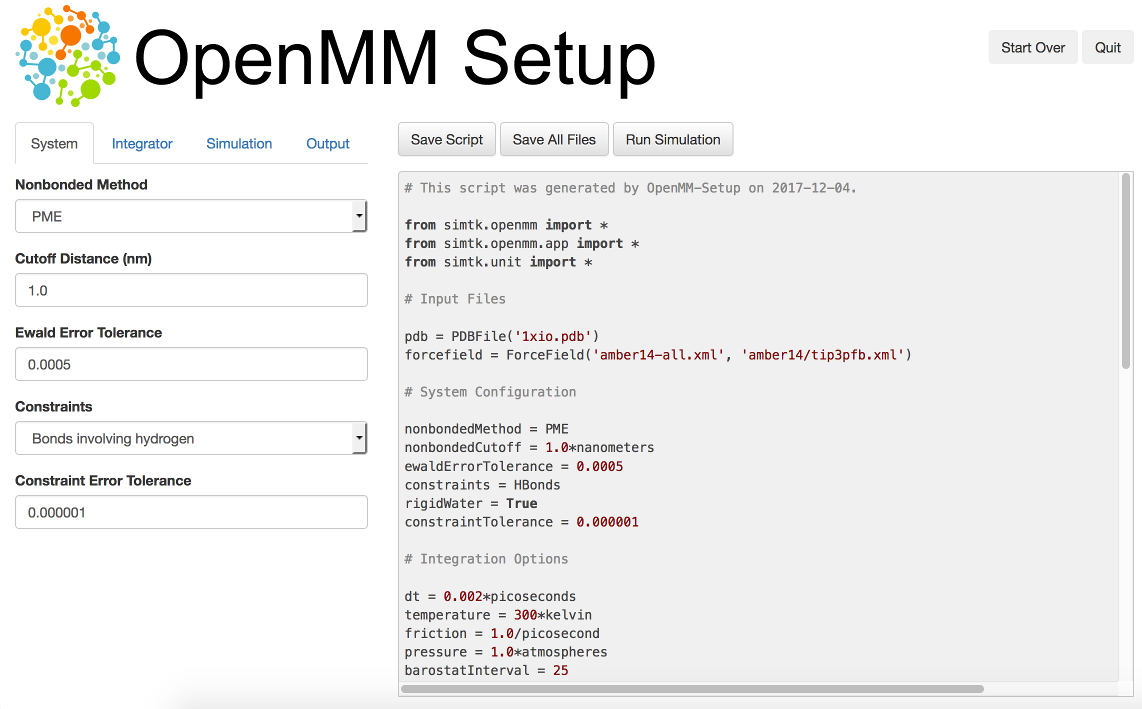
Figure 3-1: The OpenMM-Setup application
You can install OpenMM-Setup using the conda package manager with the command
conda install -c conda-forge openmm-setup
or using the pip package manager with the command
pip install openmm-setup
You can then launch it by typing the command
openmm-setup
It will automatically open a window in your web browser displaying the user interface.
OpenMM-Setup is far more than just a script generator. It can fix problems in your input files, add missing atoms, build membranes and water boxes, and much more. It is a very easy way to quickly do all necessary preparation and setup. We highly recommend it to all users of OpenMM, from novices to experts.
3.7. Simulation Parameters
Now let’s consider lots of ways you might want to customize your script.
3.7.1. Platforms
When creating a Simulation, you can optionally tell it what Platform to use.
OpenMM includes five platforms: Reference, CPU, CUDA, OpenCL, and HIP. For a
description of the differences between them, see Section 8.7. There are three ways in which
the Platform can be chosen:
1. By default, OpenMM will try to select the fastest available Platform. Usually its choice will
be reasonable, but sometimes you may want to change it.
2. Alternatively, you can set the OPENMM_DEFAULT_PLATFORM environment variable to the name
of the Platform to use. This overrides the default logic.
3. Finally, you can explicitly specify a Platform object in your script when you create the
Simulation. The following lines specify to use the CUDA platform:
platform = Platform.getPlatform('CUDA')
simulation = Simulation(prmtop.topology, system, integrator, platform)
The platform name should be one of OpenCL, CUDA, HIP, CPU, or
Reference.
You also can specify platform-specific properties that customize how calculations should be done. See Chapter 11 for details of the properties that each Platform supports. For example, the following lines specify to parallelize work across two different GPUs (CUDA devices 0 and 1), doing all computations in double precision:
platform = Platform.getPlatform('CUDA')
properties = {'DeviceIndex': '0,1', 'Precision': 'double'}
simulation = Simulation(prmtop.topology, system, integrator, platform, properties)
3.7.2. Force Fields
When you create a force field, you specify one or more XML files from which to load the force field definition. Most often, there will be one file to define the main force field, and possibly a second file to define the water model (either implicit or explicit). For example:
forcefield = ForceField('amber19-all.xml', 'amber19/tip3pfb.xml')
In some cases, one XML file may load several others. For example, amber19-all.xml
is really just a shortcut for loading several different files that together make up
the Amber19 force field. If you need finer grained control over which parameters
are loaded, you can instead specify the component files individually.
Be aware that some force fields and water models include “extra particles”, such
as lone pairs or Drude particles. Examples include the CHARMM polarizable force
field and all of the 4 and 5 site water models. To use these force fields, you
must first add the extra particles to the Topology. See section
4.4 for details.
The force fields described below are the ones that are bundled with OpenMM. Additional force fields are available online at https://github.com/openmm/openmmforcefields.
Amber19
The Amber19 force field is made up of various files that define parameters for proteins, DNA, RNA, water, and ions.
File |
Parameters |
|---|---|
|
Protein[1] |
|
DNA[2] |
|
RNA |
|
Lipid |
|
Carbohydrates and glycosylated proteins[3] |
|
TIP3P water model[4] and ions |
|
TIP3P-FB water model[5] and ions |
|
TIP4P-Ew water model[6] and ions |
|
TIP4P-FB water model[5] and ions |
|
SPC/E water model[7] and ions |
|
OPC water model[8] and ions |
|
OPC3 water model[9] and ions |
As a convenience, the file amber19-all.xml can be used as a shortcut to
include amber19/protein.ff19SB.xml, amber19/DNA.OL21.xml,
amber14/RNA.OL3.xml, and amber19/lipid21.xml. In most cases, you can simply include that file,
plus one of the water models, such as amber19/tip3pfb.xml for the
TIP3P-FB water model and ions[5]:
forcefield = ForceField('amber19-all.xml', 'amber19/tip3pfb.xml')
GLYCAM is not included by default, since it is quite large. If your system contains carbohydrates, include that file as well:
forcefield = ForceField('amber19-all.xml', 'amber19/tip3pfb.xml', 'amber14/GLYCAM_06j-1.xml')
Be aware that GLYCAM works somewhat differently from most force fields. It uses its own nonstandard naming convention for carbohydrates, and requires your input file to follow it. If any residues have names different from what it expects, GLYCAM will be unable to assign parameters to them.
Tip
Files in the amber14 directory are used by the older Amber14 force
field described below, but those also listed in the table above are shared between
the Amber14 and Amber19 force fields and can be used with the files in the
amber19 directory.
Tip
The solvent model XML files included under the amber19/ directory
include both water and ions compatible with that water model, so if you
mistakenly specify tip3p.xml instead of amber19/tip3p.xml,
you run the risk of having ForceField throw an exception since
tip3p.xml will be missing parameters for ions in your system.
The converted parameter sets come from the AmberTools 24 release and were converted using the openmmforcefields package and ParmEd.
Amber14
Similarly to the Amber19 force field, Amber14[10] is made up of
various files that define parameters for proteins, DNA, RNA, lipids, water, and
ions. The file amber14-all.xml can be used as a shortcut to include
amber14/protein.ff14SB.xml, amber14/DNA.OL15.xml,
amber14/RNA.OL3.xml, and amber14/lipid17.xml. The same remarks
for Amber19 regarding water, ions, and GLYCAM apply to Amber14.
File |
Parameters |
|---|---|
|
Protein (recommended) |
|
Protein (alternative) |
|
DNA (recommended) |
|
DNA (alternative) |
|
RNA |
|
Lipid |
|
Carbohydrates and glycosylated proteins[3] |
|
TIP3P water model[4] and ions |
|
TIP3P-FB water model[5] and ions |
|
TIP4P-Ew water model[6] and ions |
|
TIP4P-FB water model[5] and ions |
|
SPC/E water model[7] and ions |
|
OPC water model[8] and ions |
|
OPC3 water model[9] and ions |
Tip
The XML files for water and ions provided in the amber14/ directory
are identical to those in the amber19/ directory. They are provided
in both directories for compatibility and convenience.
The converted parameter sets come from the AmberTools 17 release and were converted using the openmmforcefields package and ParmEd.
CHARMM36
The CHARMM36[11] force field provides parameters for proteins, DNA, RNA, lipids, carbohydrates, water, ions, and various small molecules (see here for full references).
File |
Parameters |
|---|---|
|
Protein, DNA, RNA, lipids, carbohydrates, and small molecules |
|
Default CHARMM water model (a modified version of TIP3P[4]) and ions |
|
SPC/E water model[7] and ions |
|
TIP3P-PME-B water model[12] and ions |
|
TIP3P-PME-F water model[12] and ions |
|
TIP4P-Ew water model[6] and ions |
|
TIP4P-2005 water model[13] and ions |
|
TIP5P water model[14] and ions |
|
TIP5P-Ew water model[15] and ions |
The file charmm36_2024.xml bundles everything but the water and ions into a single
file. In most cases, you can simply include that file, plus one of the water models,
such as charmm36_2024/water.xml, which specifies the default CHARMM water model
(a modified version of TIP3P[4]) and ions:
forcefield = ForceField('charmm36_2024.xml', 'charmm36_2024/water.xml')
Tip
The solvent model XML files included under the charmm36_2024/ directory
include both water and ions compatible with that water model, so if you
mistakenly specify tip3p.xml instead of charmm36_2024/water.xml,
you run the risk of having ForceField raise an exception due to
missing parameters for ions in your system.
Tip
CHARMM makes extensive use of patches, which are automatically combined with
residue templates to create an expanded library of patched residue templates
by ForceField. That means that patched residues, such as ACE and
NME patched termini, must occur as a single residue in order for ForceField
to correctly match the residue template and apply parameters. Since these
patched residues are not standard PDB residues, Modeller does not know
how to add hydrogens to these nonstandard residues, and your input topologies
must already contain appropriate hydrogens. This can often cause problems when
trying to read in PDB files from sources such as CHARMM-GUI
that do not generate PDB files that comply with the PDB standard.
If you’re using files from CHARMM-GUI, it’s easiest to load
the PSF file directly, as discussed in Section 3.4.
Tip
Trying to read in PDB files from sources such as CHARMM-GUI
that do not generate PDB files that comply with the PDB standard
and omit CONECT records specifying bonds between residues (such as cysteines)
or include CONECT records specifying non-chemical H-H bonds in waters
can cause issues with the detection and parameter assignment for disulfide bonds.
Make sure the files you read in comply with the appropriate standards regarding
additional bonds and nonstandard residue definitions. If you’re using files from
CHARMM-GUI, it’s easiest to load
the PSF file directly, as discussed in Section 3.4.
Warning
Solvent model files in the charmm36_2024/ directory are
designed for use with charmm36_2024.xml, and those in the
charmm36/ directory are designed for use with an older
release of the CHARMM force field found in charmm36.xml and
described below. Be sure to load the correct version of the
solvent model you wish to use along with the main force field file.
Warning
Some residues and patches are not included in this port of CHARMM36, either due to a lack of support for certain CHARMM features in ParmEd, or because they generate a large number of residue-patch combinations, slowing down parameterization. The openmmforcefields package includes residues and patches not present in this port within additional force field XML files that can be loaded as needed.
The converted parameter sets come from the CHARMM36 July 2024 update, which includes the CHARMM36m protein parameters. They were converted using the openmmforcefields package and ParmEd.
Implicit Solvent
The Amber and CHARMM force fields described above can be used with any of the Generalized Born implicit solvent models from AMBER. To use them, include an extra file when creating the ForceField. For example,
forcefield = ForceField('amber19-all.xml', 'implicit/gbn2.xml')
File |
Implicit Solvent Model |
|---|---|
|
Hawkins-Cramer-Truhlar GBSA model[16] (corresponds to igb=1 in AMBER) |
|
Onufriev-Bashford-Case GBSA model[17] using the GBOBCI parameters (corresponds to igb=2 in AMBER). |
|
Onufriev-Bashford-Case GBSA model[17] using the GBOBCII parameters (corresponds to igb=5 in AMBER). |
|
GBn solvation model[18] (corresponds to igb=7 in AMBER). |
|
GBn2 solvation model[19] (corresponds to igb=8 in AMBER). |
The only nonbonded methods that are supported with implicit solvent are NoCutoff (the default),
CutoffNonPeriodic, and CutoffPeriodic. If you choose to use a nonbonded cutoff with
implicit solvent, it is usually best to set the cutoff distance larger than is typical with explicit solvent.
A cutoff of 2 nm gives good results in most cases. Periodic boundary conditions are not usually used
with implicit solvent. In fact, the lack of need for periodicity and the artifacts it creates is one
of the advantages of implicit solvent. The option is still offered, since it could be useful in some
unusual situations.
You can further control the solvation model in a few ways. First, you can specify the dielectric constants to use for the solute and solvent:
system = forcefield.createSystem(topology, soluteDielectric=1.0, solventDielectric=80.0)
If they are not specified, the solute and solvent dielectric constants default to 1.0 and 78.5, respectively.
You also can model the effect of a non-zero salt concentration by specifying the Debye-Huckel screening parameter[20]:
system = forcefield.createSystem(topology, implicitSolventKappa=1.0/nanometer)
The screening parameter can be calculated as
where \(I\) is the ionic strength in moles/liter, \(\epsilon\) is the solvent dielectric constant, and \(T\) is the temperature in Kelvin.
When one of these implicit solvent force field files is included, you can
specify the sasaMethod parameter to select a method for calculating the
solvent-accessible surface area (SASA), e.g.:
system = forcefield.createSystem(sasaMethod='LCPO')
Supported options are 'ACE' for the ACE approximation
[21][22] (which is also the default if
sasaMethod is not given), 'LCPO' for the LCPO approximation
[23], and None to disable calculation of the surface area
term entirely.
AMOEBA
The AMOEBA polarizable force field provides parameters for proteins, nucleic acids, water, and ions.
File |
Parameters |
|---|---|
|
AMOEBA 2018[24] |
|
Generalized Kirkwood solvation model[25] for use with AMOEBA 2018 force field |
|
AMOEBA 2013. This force field is deprecated. It is recommended to use AMOEBA 2018 instead. |
|
Generalized Kirkwood solvation model for use with AMOEBA 2013 force field |
|
AMOEBA 2009[26]. This force field is deprecated. It is recommended to use AMOEBA 2018 instead. |
|
Generalized Kirkwood solvation model for use with AMOEBA 2009 force field |
For explicit solvent simulations, just include the single file amoeba2018.xml.
AMOEBA also supports implicit solvent using a Generalized Kirkwood model. To enable
it, also include amoeba2018_gk.xml.
The older AMOEBA 2009 and 2013 force fields are provided only for backward compatibility, and are not recommended for most simulations.
CHARMM Polarizable Force Field
To use the CHARMM 2023 polarizable force field[27], include the
single file charmm_polar_2023.xml. It includes parameters for proteins, lipids, carbohydrates,
water, and ions. When using this force field, remember to add extra particles to
the Topology as described in section 4.4.
This force field also requires that you use one of the special integrators that
supports Drude particles. The options are DrudeLangevinIntegrator, DrudeNoseHooverIntegrator,
and DrudeSCFIntegrator.
Older Force Fields
OpenMM includes several older force fields as well. For most simulations, the newer force fields described above are preferred over any of these, but they are still useful for reproducing older results.
File |
Force Field |
|---|---|
|
Amber96[28] |
|
|
|
Amber99SB plus improved side chain torsions[31] |
|
Amber99SB with modifications to fit NMR data[32] |
|
Amber03[33] |
|
Amber10 (documented in the AmberTools manual as ff10) |
|
July 2017 release of the CHARMM36 force field without CHARMM36m protein parameters |
|
Parameters for water models and ions specifically for use with |
|
2013 version of the CHARMM polarizable force field[27] |
|
2019 version of the CHARMM polarizable force field[27] |
Several of these force fields support implicit solvent. To enable it, also include the corresponding OBC file.
File |
Implicit Solvation Model |
|---|---|
|
GBSA-OBC solvation model[17] for use with Amber96 force field |
|
GBSA-OBC solvation model for use with Amber99 force field and its variants |
|
GBSA-OBC solvation model for use with Amber03 force field |
|
GBSA-OBC solvation model for use with Amber10 force field |
Note that the GBSA-OBC parameters in these files are those used in TINKER.[34] They are designed for use with Amber force fields, but they are different from the parameters found in the AMBER application.
Water Models
The following files define popular water models. They can be used with force fields that do not provide their own water models. When using Amber19, Amber14 or CHARMM36, use the water files included with those force fields instead, since they also include ion parameters.
File |
Water Model |
|---|---|
|
TIP3P water model[4] |
|
TIP3P-FB water model[5] |
|
TIP4P-Ew water model[6] |
|
TIP4P-FB water model[5] |
|
TIP5P water model[14] |
|
SPC/E water model[7] |
|
SWM4-NDP water model[35] |
|
OPC water model[8] |
|
OPC3 water model[9] |
3.7.3. Small molecule parameters
The OpenMM force fields above include pregenerated templates for biopolymers and solvents. If your system instead contain small molecules, it is often necessary to generate these parameters on the fly.
There are two options for doing this within the OpenMM app ecosystem:
Small molecule residue template generators
One approach is to use residue template generators for small molecules from the openmmforcefields conda package. You can install this via conda with:
$ conda install -c conda-forge openmmforcefields
You can then add a small molecule residue template generator using the Open Force Field Initiative small molecule force fields using the following example:
# Create an OpenFF Molecule object for benzene from SMILES
from openff.toolkit.topology import Molecule
molecule = Molecule.from_smiles('c1ccccc1')
# Create the SMIRNOFF template generator with the default installed force field (openff-1.0.0)
from openmmforcefields.generators import SMIRNOFFTemplateGenerator
smirnoff = SMIRNOFFTemplateGenerator(molecules=molecule)
# Create an OpenMM ForceField object with AMBER ff14SB and TIP3P with compatible ions
from openmm.app import ForceField
forcefield = ForceField('amber/protein.ff14SB.xml', 'amber/tip3p_standard.xml', 'amber/tip3p_HFE_multivalent.xml')
# Register the SMIRNOFF template generator
forcefield.registerTemplateGenerator(smirnoff.generator)
Alternatively, you can use the older AMBER GAFF small molecule force field:
# Create an OpenFF Molecule object for benzene from SMILES
from openff.toolkit.topology import Molecule
molecule = Molecule.from_smiles('c1ccccc1')
# Create the GAFF template generator
from openmmforcefields.generators import GAFFTemplateGenerator
gaff = GAFFTemplateGenerator(molecules=molecule)
# Create an OpenMM ForceField object with AMBER ff14SB and TIP3P with compatible ions
from openmm.app import ForceField
forcefield = ForceField('amber/protein.ff14SB.xml', 'amber/tip3p_standard.xml', 'amber/tip3p_HFE_multivalent.xml')
# Register the GAFF template generator
forcefield.registerTemplateGenerator(gaff.generator)
# You can now parameterize an OpenMM Topology object that contains the specified molecule.
# forcefield will load the appropriate GAFF parameters when needed, and antechamber
# will be used to generate small molecule parameters on the fly.
from openmm.app import PDBFile
pdbfile = PDBFile('t4-lysozyme-L99A-with-benzene.pdb')
system = forcefield.createSystem(pdbfile.topology)
More documentation can be found on the openmmforcefields page.
Managing force fields with SystemGenerator
As an alternative to explicitly registering template generators, the openmmforcefields
package provides a SystemGenerator facility to simplify biopolymer and
small molecule force field management. To use this, you can simply specify the
small molecule force field you want to use:
# Define the keyword arguments to feed to ForceField
from openmm import unit, app
forcefield_kwargs = { 'constraints' : app.HBonds, 'rigidWater' : True, 'removeCMMotion' : False, 'hydrogenMass' : 4*unit.amu }
# Initialize a SystemGenerator using GAFF
from openmmforcefields.generators import SystemGenerator
system_generator = SystemGenerator(forcefields=['amber/ff14SB.xml', 'amber/tip3p_standard.xml'], small_molecule_forcefield='gaff-2.11', forcefield_kwargs=forcefield_kwargs, cache='db.json')
# Create an OpenMM System from an OpenMM Topology object
system = system_generator.create_system(openmm_topology)
# Alternatively, create an OpenMM System from an OpenMM Topology object and a list of OpenFF Molecule objects
molecules = Molecule.from_file('molecules.sdf', file_format='sdf')
system = system_generator.create_system(openmm_topology, molecules=molecules)
The SystemGenerator will match any instances of the molecules found in molecules.sdf to those that appear in topology.
Note that the protonation and tautomeric states must match exactly between the molecules read and those appearing in the Topology.
See the openmmforcefields documentation for more details.
3.7.4. AMBER Implicit Solvent
When creating a system from a prmtop file you do not specify force field files,
so you need a different way to tell it to use implicit solvent. This is done
with the implicitSolvent parameter:
system = prmtop.createSystem(implicitSolvent=OBC2)
OpenMM supports all of the Generalized Born models used by AMBER. Here are the
allowed values for implicitSolvent:
Value |
Meaning |
|---|---|
|
No implicit solvent is used. |
|
Hawkins-Cramer-Truhlar GBSA model[16] (corresponds to igb=1 in AMBER) |
|
Onufriev-Bashford-Case GBSA model[17] using the GBOBCI parameters (corresponds to igb=2 in AMBER). |
|
Onufriev-Bashford-Case GBSA model[17] using the GBOBCII parameters (corresponds to igb=5 in AMBER). This is the same model used by the GBSA-OBC files described in Section 3.7.2. |
|
GBn solvation model[18] (corresponds to igb=7 in AMBER). |
|
GBn2 solvation model[19] (corresponds to igb=8 in AMBER). |
You can further control the solvation model in a few ways. First, you can specify the dielectric constants to use for the solute and solvent:
system = prmtop.createSystem(implicitSolvent=OBC2, soluteDielectric=1.0,
        solventDielectric=80.0)
If they are not specified, the solute and solvent dielectrics default to 1.0 and 78.5, respectively. These values were chosen for consistency with AMBER, and are slightly different from those used elsewhere in OpenMM: when building a system from a force field, the solvent dielectric defaults to 78.3.
You also can model the effect of a non-zero salt concentration by specifying the Debye-Huckel screening parameter[20]:
system = prmtop.createSystem(implicitSolvent=OBC2, implicitSolventKappa=1.0/nanometer)
By default, OpenMM uses the ACE approximation [21][22] to the solvent-accessible surface area, but you can also use the LCPO approximation [23]:
system = prmtop.createSystem(implicitSolvent=OBC2, sasaMethod='LCPO')
This will be slower but more accurate than ACE. Specifying None for the
sasaMethod parameter will disable calculation of the surface area term
entirely.
3.7.5. Nonbonded Interactions
When creating the system (either from a force field or a prmtop file), you can specify options about how nonbonded interactions should be treated:
system = prmtop.createSystem(nonbondedMethod=PME, nonbondedCutoff=1*nanometer)
The nonbondedMethod parameter can have any of the following values:
Value |
Meaning |
|---|---|
|
No cutoff is applied. |
|
The reaction field method is used to eliminate all interactions beyond a cutoff distance. Not valid for AMOEBA. |
|
The reaction field method is used to eliminate all interactions beyond a cutoff distance. Periodic boundary conditions are applied, so each atom interacts only with the nearest periodic copy of every other atom. Not valid for AMOEBA. |
|
Periodic boundary conditions are applied. Ewald summation is used to compute long range Coulomb interactions. (This option is rarely used, since PME is much faster for all but the smallest systems.) Not valid for AMOEBA. |
|
Periodic boundary conditions are applied. The Particle Mesh Ewald method is used to compute long range Coulomb interactions. |
|
Periodic boundary conditions are applied. The Particle Mesh Ewald method is used to compute long range interactions for both Coulomb and Lennard-Jones. |
When using any method other than NoCutoff, you should also specify a
cutoff distance. Be sure to specify units, as shown in the examples above. For
example, nonbondedCutoff=1.5*nanometers or
nonbondedCutoff=12*angstroms are legal values.
When using Ewald, PME, or LJPME, you can optionally specify an
error tolerance for the force computation. For example:
system = prmtop.createSystem(nonbondedMethod=PME, nonbondedCutoff=1*nanometer,
        ewaldErrorTolerance=0.00001)
The error tolerance is roughly equal to the fractional error in the forces due to truncating the Ewald summation. If you do not specify it, a default value of 0.0005 is used.
Another optional parameter when using a cutoff is switchDistance. This
causes Lennard-Jones interactions to smoothly go to zero over some finite range,
rather than being sharply truncated at the cutoff distance. This can improve
energy conservation. To use it, specify a distance at which the interactions
should start being reduced. For example:
system = prmtop.createSystem(nonbondedMethod=PME, nonbondedCutoff=1*nanometer,
        switchDistance=0.9*nanometer)
Nonbonded Forces for AMOEBA
For the AMOEBA force field, the valid values for the nonbondedMethod
are NoCutoff and PME. The other nonbonded methods,
CutoffNonPeriodic, CutoffPeriodic, and Ewald
are unavailable for this force field.
For implicit solvent runs using AMOEBA, only the nonbondedMethod
option NoCutoff is available.
Lennard-Jones Interaction Cutoff Value
In addition, for the AMOEBA force field a cutoff for the Lennard-Jones
interaction independent of the value used for the electrostatic interactions may
be specified using the keyword vdwCutoff.
system = forcefield.createSystem(nonbondedMethod=PME, nonbondedCutoff=1*nanometer,
        ewaldErrorTolerance=0.00001, vdwCutoff=1.2*nanometer)
If vdwCutoff is not specified, then the value of
nonbondedCutoff is used for the Lennard-Jones interactions.
Specifying the Polarization Method
When using the AMOEBA force field, OpenMM allows the induced dipoles to be
calculated in any of three different ways. The slowest but potentially most
accurate method is to iterate the calculation until the dipoles converge to a
specified tolerance. To select this, specify polarization='mutual'.
Use the mutualInducedTargetEpsilon option to select the tolerance; for
most situations, a value of 0.00001 works well. Alternatively you can specify
polarization='extrapolated'. This uses an analytic approximation
[36] to estimate what the fully converged dipoles will be without
actually continuing the calculation to convergence. In many cases this can be
significantly faster with only a small loss in accuracy. Finally, you can
specify polarization='direct' to use the direct polarization
approximation, in which induced dipoles depend only on the fixed multipoles, not
on other induced dipoles. This is even faster, but it produces very different
forces from mutual polarization, so it should only be used with force fields
that have been specifically parameterized for use with this approximation.
Here are examples of using each method:
system = forcefield.createSystem(nonbondedMethod=PME, nonbondedCutoff=1*nanometer,
    vdwCutoff=1.2*nanometer, polarization='mutual', mutualInducedTargetEpsilon=0.00001)

system = forcefield.createSystem(nonbondedMethod=PME, nonbondedCutoff=1*nanometer,
    vdwCutoff=1.2*nanometer, polarization='extrapolated')

system = forcefield.createSystem(nonbondedMethod=PME, nonbondedCutoff=1*nanometer,
    vdwCutoff=1.2*nanometer, polarization='direct')
Implicit Solvent and Solute Dielectrics
For implicit solvent simulations using the AMOEBA force field, the
amoeba2013_gk.xml file should be included in the initialization of the force
field:
forcefield = ForceField('amoeba2009.xml', 'amoeba2009_gk.xml')
Only the nonbondedMethod option NoCutoff is available
for implicit solvent runs using AMOEBA. In addition, the solvent and solute
dielectric values can be specified for implicit solvent simulations:
system=forcefield.createSystem(nonbondedMethod=NoCutoff, soluteDielectric=2.0,
        solventDielectric=80.0)
The default values are 1.0 for the solute dielectric and 78.3 for the solvent dielectric.
3.7.6. Constraints
When creating the system (either from a force field or an AMBER prmtop file), you can
optionally tell OpenMM to constrain certain bond lengths and angles. For
example,
system = prmtop.createSystem(nonbondedMethod=NoCutoff, constraints=HBonds)
The constraints parameter can have any of the following values:
Value |
Meaning |
|---|---|
|
No constraints are applied. This is the default value. |
|
The lengths of all bonds that involve a hydrogen atom are constrained. |
|
The lengths of all bonds are constrained. |
|
The lengths of all bonds are constrained. In addition, all angles of the form H-X-H or H-O-X (where X is an arbitrary atom) are constrained. |
The main reason to use constraints is that it allows one to use a larger
integration time step. With no constraints, one is typically limited to a time
step of about 1 fs for typical biomolecular force fields like AMBER or CHARMM.
With HBonds constraints, this can be increased to about 2 fs for Verlet
dynamics, or about 4 fs for Langevin dynamics. With HAngles, it can
sometimes be increased even further.
Regardless of the value of this parameter, OpenMM makes water molecules
completely rigid, constraining both their bond lengths and angles. You can
disable this behavior with the rigidWater parameter:
system = prmtop.createSystem(nonbondedMethod=NoCutoff, constraints=None, rigidWater=False)
Be aware that flexible water may require you to further reduce the integration step size, typically to about 0.5 fs.
Note
The AMOEBA forcefield is designed to be used without constraints, so by
default OpenMM makes AMOEBA water flexible. You can still force it to be
rigid by specifying rigidWater=True.
3.7.7. Heavy Hydrogens
When creating the system (either from a force field or an AMBER prmtop file), you can
optionally tell OpenMM to increase the mass of hydrogen atoms. For example,
system = prmtop.createSystem(hydrogenMass=4*amu)
This applies only to hydrogens that are bonded to heavy atoms, and any mass
added to the hydrogen is subtracted from the heavy atom. This keeps their total
mass constant while slowing down the fast motions of hydrogens. When combined
with constraints (typically constraints=AllBonds), this often allows a
further increase in integration step size.
3.7.8. Integrators
OpenMM offers a choice of several different integration methods. You select which one to use by creating an integrator object of the appropriate type. Detailed descriptions of all these integrators can be found in Chapter 21. In addition to these built in integrators, lots of others are available as part of the OpenMMTools package.
Langevin Middle Integrator
In the examples of the previous sections, we used Langevin integration:
integrator = LangevinMiddleIntegrator(300*kelvin, 1/picosecond, 0.004*picoseconds)
The three parameter values in this line are the simulation temperature (300 K),
the friction coefficient (1 ps-1), and the step size (0.004 ps). You
are free to change these to whatever values you want. Be sure to specify units
on all values. For example, the step size could be written either as
0.004*picoseconds or 4*femtoseconds. They are exactly
equivalent. Note that LangevinMiddleIntegrator is a leapfrog
integrator, so the velocities are offset by half a time step from the positions.
Langevin Integrator
LangevinIntegrator is very similar to LangevinMiddleIntegrator,
but it uses a different discretization of the Langevin equation.
LangevinMiddleIntegrator tends to produce more accurate configurational
sampling, and therefore is preferred for most applications. Also note that
LangevinIntegrator, like LangevinMiddleIntegrator, is a leapfrog
integrator, so the velocities are offset by half a time step from the positions.
Nosé-Hoover Integrator
The NoseHooverIntegrator uses the same “middle” leapfrog propagation
algorithm as LangevinMiddleIntegrator, but replaces the stochastic
temperature control with a velocity scaling algorithm that produces more
accurate transport properties [37]. This velocity scaling
results from propagating a chain of extra variables, which slightly reduces the
computational efficiency with respect to LangevinMiddleIntegrator. The
thermostated integrator is minimally created with syntax analogous to the
LangevinMiddleIntegrator example above:
NoseHooverIntegrator integrator(300*kelvin, 1/picosecond,
                                0.004*picoseconds);
The first argument specifies the target temperature. The second specifies the frequency of interaction with the heat bath: a lower value interacts minimally, yielding the microcanonical ensemble in the limit of a zero frequency, while a larger frequency will perturb the system greater, keeping it closer to the target temperature. The third argument is the integration timestep that, like the other arguments, must be specified with units. For initial equilibration to the target temperature, a larger interaction frequency is recommended, e.g. 25 ps-1.
This integrator supports lots of other options, including the ability to couple different parts of the system to thermostats at different temperatures. See the API documentation for details.
Leapfrog Verlet Integrator
A leapfrog Verlet integrator can be used for running constant energy dynamics. The command for this is:
integrator = VerletIntegrator(0.002*picoseconds)
The only option is the step size.
Brownian Integrator
Brownian (diffusive) dynamics can be used by specifying the following:
integrator = BrownianIntegrator(300*kelvin, 1/picosecond, 0.002*picoseconds)
The parameters are the same as for Langevin dynamics: temperature (300 K), friction coefficient (1 ps-1), and step size (0.002 ps).
Variable Time Step Langevin Integrator
A variable time step Langevin integrator continuously adjusts its step size to keep the integration error below a specified tolerance. In some cases, this can allow you to use a larger average step size than would be possible with a fixed step size integrator. It also is very useful in cases where you do not know in advance what step size will be stable, such as when first equilibrating a system. You create this integrator with the following command:
integrator = VariableLangevinIntegrator(300*kelvin, 1/picosecond, 0.001)
In place of a step size, you specify an integration error tolerance (0.001 in this example). It is best not to think of this value as having any absolute meaning. Just think of it as an adjustable parameter that affects the step size and integration accuracy. Smaller values will produce a smaller average step size. You should try different values to find the largest one that produces a trajectory sufficiently accurate for your purposes.
Variable Time Step Leapfrog Verlet Integrator
A variable time step leapfrog Verlet integrator works similarly to the variable time step Langevin integrator in that it continuously adjusts its step size to keep the integration error below a specified tolerance. The command for this integrator is:
integrator = VariableVerletIntegrator(0.001)
The parameter is the integration error tolerance (0.001), whose meaning is the same as for the Langevin integrator.
Multiple Time Step Integrator
The MTSIntegrator class implements the rRESPA multiple time step
algorithm[38]. This allows some forces in the system to be evaluated more
frequently than others. For details on how to use it, consult the API
documentation.
Multiple Time Step Langevin Integrator
MTSLangevinIntegrator is similar to MTSIntegrator, but it uses
the Langevin method to perform constant temperature dynamics. For details on
how to use it, consult the API documentation.
Compound Integrator
The CompoundIntegrator class is useful for cases where you want to use
multiple integration algorithms within a single simulation. It allows you to
create multiple integrators, then switch back and forth between them. For
details on how to use it, consult the API documentation.
3.7.9. Temperature Coupling
If you want to run a simulation at constant temperature, using a Langevin integrator (as shown in the examples above) is usually the best way to do it. OpenMM does provide an alternative, however: you can use a Verlet integrator, then add an Andersen thermostat to your system to provide temperature coupling.
To do this, we can add an AndersenThermostat object to the System as shown below.
...
system = prmtop.createSystem(nonbondedMethod=PME, nonbondedCutoff=1*nanometer,
        constraints=HBonds)
system.addForce(AndersenThermostat(300*kelvin, 1/picosecond))
integrator = VerletIntegrator(0.002*picoseconds)
...
The two parameters of the Andersen thermostat are the temperature (300 K) and collision frequency (1 ps-1).
3.7.10. Pressure Coupling
All the examples so far have been constant volume simulations. If you want to run at constant pressure instead, add a Monte Carlo barostat to your system. You do this exactly the same way you added the Andersen thermostat in the previous section:
...
system = prmtop.createSystem(nonbondedMethod=PME, nonbondedCutoff=1*nanometer,
        constraints=HBonds)
system.addForce(MonteCarloBarostat(1*bar, 300*kelvin))
integrator = LangevinMiddleIntegrator(300*kelvin, 1/picosecond, 0.004*picoseconds)
...
The parameters of the Monte Carlo barostat are the pressure (1 bar) and temperature (300 K). The barostat assumes the simulation is being run at constant temperature, but it does not itself do anything to regulate the temperature.
Warning
It is therefore critical that you always use it along with a Langevin integrator or Andersen thermostat, and that you specify the same temperature for both the barostat and the integrator or thermostat. Otherwise, you will get incorrect results.
There also is an anisotropic barostat that scales each axis of the periodic box independently, allowing it to change shape. When using the anisotropic barostat, you can specify a different pressure for each axis. The following line applies a pressure of 1 bar along the X and Y axes, but a pressure of 2 bar along the Z axis:
system.addForce(MonteCarloAnisotropicBarostat((1, 1, 2)*bar, 300*kelvin))
Another feature of the anisotropic barostat is that it can be applied to only certain axes of the periodic box, keeping the size of the other axes fixed. This is done by passing three additional parameters that specify whether the barostat should be applied to each axis. The following line specifies that the X and Z axes of the periodic box should not be scaled, so only the Y axis can change size.
system.addForce(MonteCarloAnisotropicBarostat((1, 1, 1)*bar, 300*kelvin,
        False, True, False))
There is a third barostat designed specifically for simulations of membranes. It assumes the membrane lies in the XY plane, and treats the X and Y axes of the box differently from the Z axis. It also applies a uniform surface tension in the plane of the membrane. The following line adds a membrane barostat that applies a pressure of 1 bar and a surface tension of 200 bar*nm. It specifies that the X and Y axes are treated isotropically while the Z axis is free to change independently.
system.addForce(MonteCarloMembraneBarostat(1*bar, 200*bar*nanometer,
    MonteCarloMembraneBarostat.XYIsotropic, MonteCarloMembraneBarostat.ZFree, 300*kelvin))
See the API documentation for details about the allowed parameter values and their meanings.
3.7.11. Energy Minimization
As seen in the examples, performing a local energy minimization takes a single line in the script:
simulation.minimizeEnergy()
In most cases, that is all you need. There are two optional parameters you can specify if you want further control over the minimization. First, you can specify a tolerance for when the energy should be considered to have converged:
simulation.minimizeEnergy(tolerance=5*kilojoule/mole/nanometer)
If you do not specify this parameter, a default tolerance of 10 kilojoule/mole/nanometer is used.
Second, you can specify a maximum number of iterations:
simulation.minimizeEnergy(maxIterations=100)
The minimizer will exit once the specified number of iterations is reached, even if the energy has not yet converged. If you do not specify this parameter, the minimizer will continue until convergence is reached, no matter how many iterations it takes.
These options are independent. You can specify both if you want:
simulation.minimizeEnergy(tolerance=0.1*kilojoule/mole/nanometer, maxIterations=500)
3.7.12. Removing Center of Mass Motion
By default, System objects created with the OpenMM application tools add
a CMMotionRemover that removes all center of mass motion at every time step so the
system as a whole does not drift with time. This is almost always what you
want. In rare situations, you may want to allow the system to drift with time.
You can do this by specifying the removeCMMotion parameter when you
create the System:
system = forcefield.createSystem(pdb.topology, nonbondedMethod=NoCutoff,
        removeCMMotion=False)
3.7.13. Writing Trajectories
OpenMM can save simulation trajectories to disk in four formats: PDB, PDBx/mmCIF, DCD and XTC. All of these are widely supported formats, so you should be able to read them into most analysis and visualization programs.
To save a trajectory, just add a “reporter” to the simulation, as shown in the example scripts above:
simulation.reporters.append(DCDReporter('output.dcd', 1000))
The two parameters of the DCDReporter are the output filename and how often (in
number of time steps) output structures should be written. To use PDB, PDBx/mmCIF,
or XTC format, just replace DCDReporter with PDBReporter, PDBxReporter,
or XTCReporter. The parameters represent the same values:
simulation.reporters.append(XTCReporter('output.xtc', 1000))
3.7.14. Recording Other Data
In addition to saving a trajectory, you may want to record other information
over the course of a simulation, such as the potential energy or temperature.
OpenMM provides a reporter for this purpose also. Create a StateDataReporter
and add it to the simulation:
simulation.reporters.append(StateDataReporter('data.csv', 1000, time=True,
        kineticEnergy=True, potentialEnergy=True))
The first two parameters are the output filename and how often (in number of
time steps) values should be written. The remaining arguments specify what
values should be written at each report. The available options are
step (the index of the current time step), time,
progress (what percentage of the simulation has completed),
remainingTime (an estimate of how long it will take the simulation to
complete), potentialEnergy, kineticEnergy,
totalEnergy, temperature, volume (the volume
of the periodic box), density (the total system mass divided by the
volume of the periodic box), and speed (an estimate of how quickly
the simulation is running). If you include either the progress or
remainingTime option, you must also include the totalSteps
parameter to specify the total number of time steps that will be included in the
simulation. One line is written to the file for each report containing the
requested values. By default the values are written in comma-separated-value
(CSV) format. You can use the separator parameter to choose a
different separator. For example, the following line will cause values to be
separated by spaces instead of commas:
simulation.reporters.append(StateDataReporter('data.txt', 1000, progress=True,
        temperature=True, totalSteps=10000, separator=' '))
3.7.15. Saving Simulation Progress and Results
There are three built-in ways to save the results of your simulation in OpenMM
(additional methods can be written yourself or imported through other packages
like mdtraj or parmed). If you are simply interested in saving the structure,
you can write it out as a PDB file using PDBFile.writeFile(). You can
see an example of this in the modeller section 4.6.
If you are hoping to save more information than just positions, you can use
simulation.saveState(). This will save the entire state of the
simulation, including positions, velocities, box dimensions and much more in an
XML file. This same file can be loaded back into OpenMM and used to continue
the simulation. Importantly, because this file is a text file, it can be
transfered between different platforms and different versions of OpenMM. A
potential downside to this approach is that state files are often quite large,
and may not fit all use cases. Here’s an example of how to use it:
simulation.saveState('output.xml')
To load the simulation back in:
simulation.loadState('output.xml')
There is a third way to save your simulation, known as a checkpoint file, which will save the entire simulation as a binary file. It will allow you to exactly continue a simulation if the need arises (though whether the simulation is deterministic depends on platform and methods, see 11.5). There are important caveats to this approach, however. This binary can only be used to restart simulations on machines with the same hardware and the same OpenMM version as the one that saved it. Therefore, it should only be used when it’s clear that won’t be an issue.
simulation.saveCheckpoint('state.chk')
And can be loaded back in like this:
simulation.loadCheckpoint('state.chk')
Finally, OpenMM comes with a built-in reporter for saving checkpoints, the
CheckpointReporter, which can be helpful in restarting simulations
that failed unexpectedly or due to outside reasons (e.g. server crash). To save
a checkpoint file every 5,000 steps, for example:
simulation.reporters.append(CheckpointReporter('checkpnt.chk', 5000))
Note that the checkpoint reporter will overwrite the last checkpoint file.
3.7.16. Enhanced Sampling Methods
In many situations, the goal of a simulation is to sample the range of configurations accessible to a system. It does not matter whether the simulation represents a single, physically realistic trajectory, only whether it produces a correct distribution of states. In this case, a variety of methods can be used to sample configuration space much more quickly and efficiently than a single physical trajectory would. These are known as enhanced sampling methods. OpenMM offers several that you can choose from. They are briefly described here. Consult the API documentation for more detailed descriptions and example code.
Simulated Tempering
Simulated tempering[39] involves making frequent changes to the temperature of a simulation. At high temperatures, it can quickly cross energy barriers and explore a wide range of configurations. At lower temperatures, it more thoroughly explores each local region of configuration space. This is a powerful method to speed up sampling when you do not know in advance what motions you want to sample. Simply specify the range of temperatures to simulate and the algorithm handles everything for you mostly automatically.
Metadynamics
Metadynamics[40] is used when you do know in advance what motions you want to sample. You specify one or more collective variables, and the algorithm adds a biasing potential to make the simulation explore a wide range of values for those variables. It does this by periodically adding “bumps” to the biasing potential at the current values of the collective variables. This encourages the simulation to move away from regions it has already explored and sample a wide range of values. At the end of the simulation, the biasing potential can be used to calculate the free energy of the system as a function of the collective variables.
Accelerated Molecular Dynamics (aMD)
aMD[41] is another method that can be used when you do not know in
advance what motions you want to accelerate. It alters the potential energy surface
by adding a “boost” potential whenever the potential energy is below a threshold.
This makes local minima shallower and allows more frequent transitions between them.
The boost can be applied to the total potential energy, to just a subset of interactions
(typically the dihedral torsions), or both. There are separate integrator classes
for each of these options: AMDIntegrator, AMDForceGroupIntegrator,
and DualAMDIntegrator.