10. OpenMM C++ API Examples
This chapter describes examples provided with OpenMM demonstrating how to use the OpenMM C++ API (as well as the C and Fortran API wrappers).
10.1. Example Files Overview
Four example files are provided in the examples/cpp-examples folder,
each designed with a specific objective.
HelloArgon: A very simple example intended for verifying that you have installed OpenMM correctly. It also introduces you to the basic classes within OpenMM.
HelloSodiumChloride: This example shows you our recommended strategy for integrating OpenMM into an existing molecular dynamics code.
HelloEthane: The main purpose of this example is to demonstrate how to tell OpenMM about bonded forces (bond stretch, bond angle bend, dihedral torsion).
HelloWaterBox: This example shows you how to use OpenMM to model explicit solvation, including setting up periodic boundary conditions. It runs extremely fast on a GPU but very, very slowly on a CPU, so it is an excellent example to use to compare performance on the GPU versus the CPU. The other examples provided use systems where the performance difference would be too small to notice.
The two fundamental examples—HelloArgon and HelloSodiumChloride—are provided in C++, C, and Fortran, as indicated in the table below. The other two examples—HelloEthane and HelloWaterBox—follow the same structure as HelloSodiumChloride but demonstrate more calls within the OpenMM API. They are only provided in C++ but can be adapted to run in C and Fortran by following the mappings described in Chapter 12. HelloArgon and HelloSodiumChloride also serve as examples of how to do these mappings. The sections below describe the HelloArgon, HelloSodiumChloride, and HelloEthane programs in more detail.
Example |
Solvent |
Thermostat |
Boundary |
Forces & Constraints |
API |
|---|---|---|---|---|---|
Argon |
Vacuum |
None |
None |
Non-bonded* |
C++, C, Fortran |
Sodium Chloride |
Implicit water |
Langevin |
None |
Non-bonded* |
C++, C, Fortran |
Ethane |
Vacuum |
None |
None |
Non-bonded*, stretch, bend, torsion |
C++ |
Water Box |
Explicit water |
Andersen |
Periodic |
Non-bonded*, stretch, bend, constraints |
C++ |
*van der Waals and Coulomb forces
10.2. Running Example Files
The instructions below are for running the HelloArgon program. A similar process would be used to run the other examples.
10.2.1. Visual Studio
Navigate to wherever you saved the example files. Descend into the directory folder VisualStudio. Double-click the file HelloArgon.sln (a Microsoft Visual Studio Solution file). Visual Studio will launch.
Note: These files were created using Visual Studio 8. If you are using a more recent version, it will ask if you want to convert the files to the new version. Agree and continue through the conversion process.
In Visual Studio, make sure the “Solution Configuration” is set to “Release” and not “Debug”. The “Solution Configuration” can be set using the drop-down menu in the top toolbar, next to the green arrow (see Figure 10-1 below). Due to incompatibilities among Visual Studio versions, we do not provide pre-compiled debug binaries.
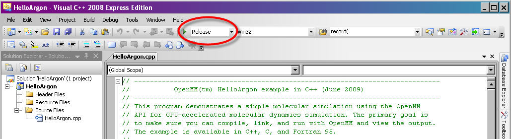
Figure 10-1: Setting “Solution Configuration” to “Release” mode in Visual Studio
From the command options select Debug -> Start Without Debugging (or CTRL-F5). See Figure 10-2. This will also compile the program, if it has not previously been compiled.
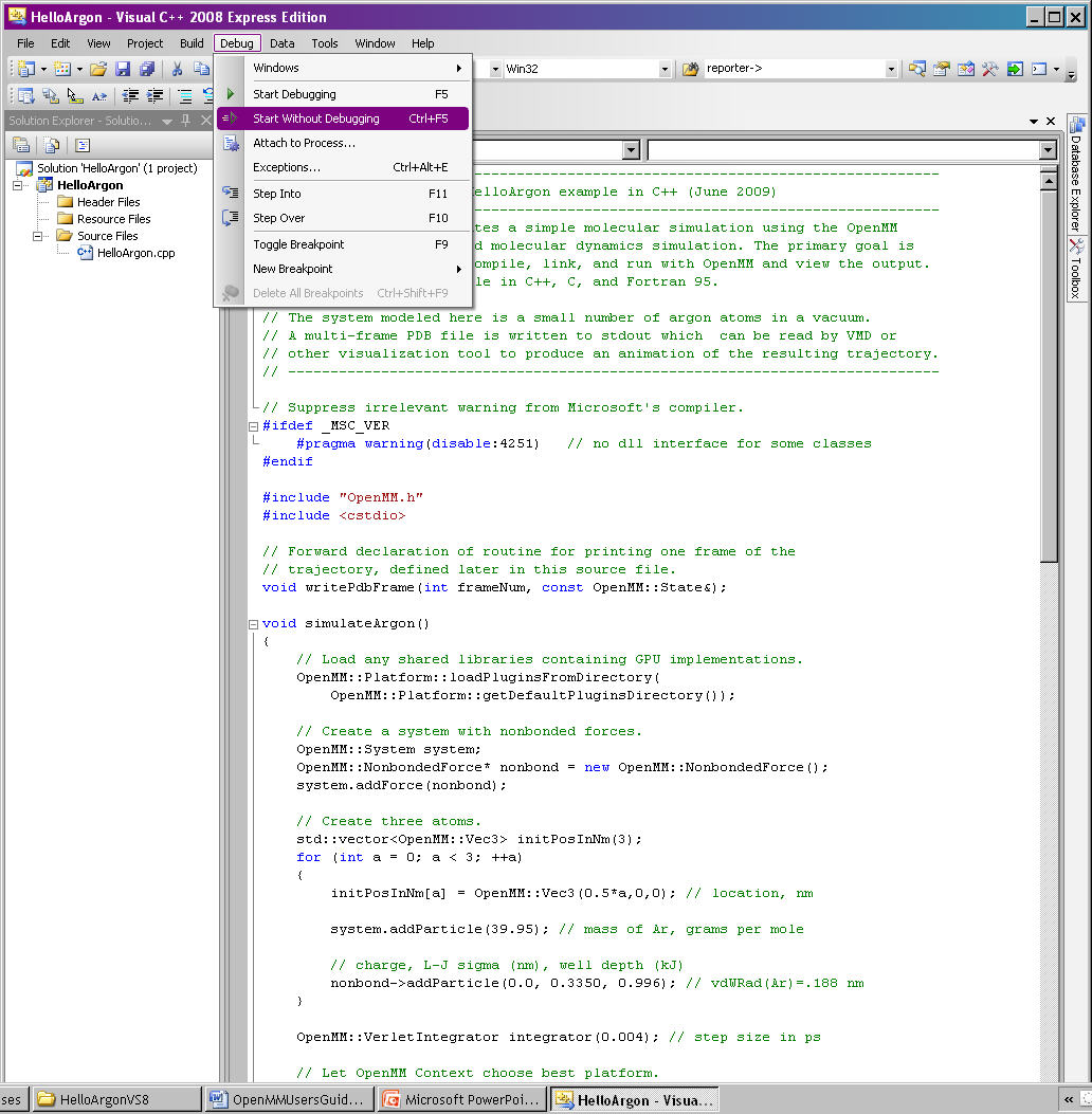
Figure 10-2: Run a program in Visual Studio
You should see a series of lines like the following output on your screen:
REMARK  Using OpenMM platform Reference
MODEL     1
ATOM      1  AR   AR     1       0.000   0.000   0.000  1.00  0.00
ATOM      2  AR   AR     1       5.000   0.000   0.000  1.00  0.00
ATOM      3  AR   AR     1       10.000  0.000   0.000  1.00  0.00
ENDMDL

…

MODEL     250
ATOM      1  AR   AR     1       0.233   0.000   0.000  1.00  0.00
ATOM      2  AR   AR     1       5.068   0.000   0.000  1.00  0.00
ATOM      3  AR   AR     1       9.678   0.000   0.000  1.00  0.00
ENDMDL
MODEL     251
ATOM      1  AR   AR     1       0.198   0.000   0.000  1.00  0.00
ATOM      2  AR   AR     1       5.082   0.000   0.000  1.00  0.00
ATOM      3  AR   AR     1       9.698   0.000   0.000  1.00  0.00
ENDMDL
MODEL     252
ATOM      1  AR   AR     1       0.165   0.000   0.000  1.00  0.00
ATOM      2  AR   AR     1       5.097   0.000   0.000  1.00  0.00
ATOM      3  AR   AR     1       9.717   0.000   0.000  1.00  0.00
ENDMDL
Determining the platform being used
The very first line of the output will indicate whether you are running on the CPU (Reference platform) or a GPU (CUDA or OpenCL platform). It will say one of the following:
REMARK  Using OpenMM platform Reference
REMARK  Using OpenMM platform Cuda
REMARK  Using OpenMM platform OpenCL
If you have a supported GPU, the program should, by default, run on the GPU.
Visualizing the results
You can output the results to a PDB file that could be visualized using programs like VMD (http://www.ks.uiuc.edu/Research/vmd/) or PyMol (https://www.pymol.org). To do this within Visual Studios:
Right-click on the project name HelloArgon (not one of the files) and select the “Properties” option.
On the “Property Pages” form, select “Debugging” under the “Configuration Properties” node.
In the “Command Arguments” field, type:
> argon.pdb
This will save the output to a file called argon.pdb in the current working directory (default is the VisualStudio directory). If you want to save it to another directory, you will need to specify the full path.
Select “OK”
Now, when you run the program in Visual Studio, no text will appear. After a
short time, you should see the message “Press any key to continue…,”
indicating that the program is complete and that the PDB file has been
completely written.
10.2.2. Mac OS X/Linux
Navigate to wherever you saved the example files.
Verify your makefile by consulting the MakefileNotes file in this directory, if necessary.
Type::
make
Then run the program by typing:
./HelloArgon
You should see a series of lines like the following output on your screen:
REMARK  Using OpenMM platform Reference
MODEL     1
ATOM      1  AR   AR     1       0.000   0.000   0.000  1.00  0.00
ATOM      2  AR   AR     1       5.000   0.000   0.000  1.00  0.00
ATOM      3  AR   AR     1       10.000  0.000   0.000  1.00  0.00
ENDMDL

...

MODEL     250
ATOM      1  AR   AR     1       0.233   0.000   0.000  1.00  0.00
ATOM      2  AR   AR     1       5.068   0.000   0.000  1.00  0.00
ATOM      3  AR   AR     1       9.678   0.000   0.000  1.00  0.00
ENDMDL
MODEL     251
ATOM      1  AR   AR     1       0.198   0.000   0.000  1.00  0.00
ATOM      2  AR   AR     1       5.082   0.000   0.000  1.00  0.00
ATOM      3  AR   AR     1       9.698   0.000   0.000  1.00  0.00
ENDMDL
MODEL     252
ATOM      1  AR   AR     1       0.165   0.000   0.000  1.00  0.00
ATOM      2  AR   AR     1       5.097   0.000   0.000  1.00  0.00
ATOM      3  AR   AR     1       9.717   0.000   0.000  1.00  0.00
ENDMDL
Determining the platform being used
The very first line of the output will indicate whether you are running on the CPU (Reference platform) or a GPU (CUDA or OpenCL platform). It will say one of the following:
REMARK  Using OpenMM platform Reference
REMARK  Using OpenMM platform Cuda
REMARK  Using OpenMM platform OpenCL
If you have a supported GPU, the program should, by default, run on the GPU.
Visualizing the results
You can output the results to a PDB file that could be visualized using programs like VMD (http://www.ks.uiuc.edu/Research/vmd/) or PyMol (https://www.pymol.org) by typing:
./HelloArgon > argon.pdb
Compiling Fortran and C examples
The Makefile provided with the examples can also be used to compile the Fortran and C examples.
The Fortran compiler needs to load a version of the libstdc++.dylib library that
is compatible with the version of gcc used to build OpenMM; OpenMM for Mac is
compiled using gcc 4.2. If you are compiling with a different version, edit the
Makefile and add the following flag to FCPPLIBS: -L/usr/lib/gcc/i686
-apple-darwin10/4.2.1.
When the Makefile has been updated, type:
make all
10.3. HelloArgon Program
The HelloArgon program simulates three argon atoms in a vacuum. It is a simple program primarily intended for you to verify that you are able to compile, link, and run with OpenMM. It also demonstrates the basic calls needed to run a simulation using OpenMM.
10.3.1. Including OpenMM-defined functions
The OpenMM header file OpenMM.h instructs the program to include everything defined by the OpenMM libraries. Include the header file by adding the following line at the top of your program:
#include "OpenMM.h"
10.3.2. Running a program on GPU platforms
By default, a program will run on the Reference platform. In order to run a program on another platform (e.g., an NVIDIA or AMD GPU), you need to load the required shared libraries for that other platform (e.g., Cuda, OpenCL). The easy way to do this is to call:
OpenMM::Platform::loadPluginsFromDirectory(OpenMM::Platform::getDefaultPluginsDirectory());
This will load all the shared libraries (plug-ins) that can be found, so you do not need to explicitly know which libraries are available on a given machine. In this way, the program will be able to run on another platform, if it is available.
10.3.3. Running a simulation using the OpenMM public API
The OpenMM public API was described in Section 8.5. Here you will
see how to use those classes to create a simple system of three argon atoms and run a short
simulation. The main components of the simulation are within the function
simulateArgon():
System – We first establish a system and add a non-bonded force to it. At this point, there are no particles in the system.
// Create a system with nonbonded forces.
OpenMM::System system;
OpenMM::NonbondedForce* nonbond = new OpenMM::NonbondedForce();
system.addForce(nonbond);
We then add the three argon atoms to the system. For this system, all the data for the particles are hard-coded into the program. While not a realistic scenario, it makes the example simpler and clearer. The
std::vector<OpenMM::Vec3>is an array of vectors of 3.// Create three atoms. std::vector<OpenMM::Vec3> initPosInNm(3); for (int a = 0; a < 3; ++a) { initPosInNm[a] = OpenMM::Vec3(0.5*a,0,0); // location, nm system.addParticle(39.95); // mass of Ar, grams per mole // charge, L-J sigma (nm), well depth (kJ) nonbond->addParticle(0.0, 0.3350, 0.996); // vdWRad(Ar)=.188 nm }
Units: Be very careful with the units in your program. It is very easy to make mistakes with the units, so we recommend including them in your variable names, as we have done here
initPosInNm(position in nanometers). OpenMM provides conversion constants that should be used whenever there are conversions to be done; for simplicity, we did not do that in HelloArgon, but all the other examples show the use of these constants.It is hard to overemphasize the importance of careful units handling—it is very easy to make a mistake despite, or perhaps because of, the trivial nature of units conversion. For more information about the units used in OpenMM, see Section 18.2.
Adding Particle Information: Both the system and the non-bonded force require information about the particles. The system just needs to know the mass of the particle. The non-bonded force requires information about the charge (in this case, argon is uncharged), and the Lennard-Jones parameters sigma (zero-energy separation distance) and well depth (see Section 19.6.1 for more details).
Note that the van der Waals radius for argon is 0.188 nm and that it has already been converted to sigma (0.335 nm) in the example above where it is added to the non-bonded force; in your code, you should make use of the appropriate conversion factor supplied with OpenMM as discussed in Section 18.2.
Integrator – We next specify the integrator to use to perform the calculations. In this case, we choose a Verlet integrator to run a constant energy simulation. The only argument required is the step size in picoseconds.
OpenMM::VerletIntegrator integrator(0.004); // step size in ps
We have chosen to use 0.004 picoseconds, or 4 femtoseconds, which is larger than that used in a typical molecular dynamics simulation. However, since this example does not have any bonds with higher frequency components, like most molecular dynamics simulations do, this is an acceptable value.
Context – The context is an object that consists of an integrator and a system. It manages the state of the simulation. The code below initializes the context. We then let the context select the best platform available to run on, since this is not specifically specified, and print out the chosen platform. This is useful information, especially when debugging.
// Let OpenMM Context choose best platform.
OpenMM::Context context(system, integrator);
printf("REMARK  Using OpenMM platform %s\n", context.getPlatform().getName().c_str());
We then initialize the system, setting the initial time, as well as the initial positions and velocities of the atoms. In this example, we leave time and velocity at their default values of zero.
// Set starting positions of the atoms. Leave time and velocity zero.
context.setPositions(initPosInNm);
Initialize and run the simulation – The next block of code runs the simulation and saves its output. For each frame of the simulation (in this example, a frame is defined by the advancement interval of the integrator; see below), the current state of the simulation is obtained and written out to a PDB-formatted file.
// Simulate.
for (int frameNum=1; ;++frameNum) {
    // Output current state information.
    OpenMM::State state = context.getState(OpenMM::State::Positions);
    const double  timeInPs = state.getTime();
    writePdbFrame(frameNum, state); // output coordinates
Getting state information has to be done in bulk, asking for information for all the particles at once. This is computationally expensive since this information can reside on the GPUs and requires communication overhead to retrieve, so you do not want to do it very often. In the above code, we only request the positions, since that is all that is needed, and time from the state.
The simulation stops after 10 ps; otherwise we ask the integrator to take 10 steps (so one frame is equivalent to 10 time steps). Normally, we would want to take more than 10 steps at a time, but to get a reasonable-looking animation, we use 10.
if (timeInPs >= 10.)
    break;

// Advance state many steps at a time, for efficient use of OpenMM.
integrator.step(10); // (use a lot more than this normally)
10.3.4. Error handling for OpenMM
Error handling for OpenMM is explicitly designed so you do not have to check the
status after every call. If anything goes wrong, OpenMM throws an exception.
It uses standard exceptions, so on many platforms, you will get the exception
message automatically. However, we recommend using try-catch blocks
to ensure you do catch the exception.
int main()
{
    try {
        simulateArgon();
        return 0; // success!
    }
    // Catch and report usage and runtime errors detected by OpenMM and fail.
    catch(const std::exception& e) {
        printf("EXCEPTION: %s\n", e.what());
        return 1; // failure!
    }
}
10.3.5. Writing out PDB files
For the HelloArgon program, we provide a simple PDB file writing function
writePdbFrame that only writes out argon atoms. The function
has nothing to do with OpenMM except for using the OpenMM State. The function
extracts the positions from the State in nanometers (10-9 m) and
converts them to Angstroms (10-10 m) to be compatible with the PDB
format. Again, we emphasize how important it is to track the units being used!
void writePdbFrame(int frameNum, const OpenMM::State& state)
{
    // Reference atomic positions in the OpenMM State.
    const std::vector<OpenMM::Vec3>& posInNm = state.getPositions();

    // Use PDB MODEL cards to number trajectory frames
    printf("MODEL     %d\n", frameNum); // start of frame
    for (int a = 0; a < (int)posInNm.size(); ++a)
    {
        printf("ATOM  %5d  AR   AR     1    ", a+1); // atom number
        printf("%8.3f%8.3f%8.3f  1.00  0.00\n",      // coordinates
        // "*10" converts nanometers to Angstroms
        posInNm[a][0]*10, posInNm[a][1]*10, posInNm[a][2]*10);
    }
    printf("ENDMDL\n"); // end of frame
}
MODEL and ENDMDL are used to mark the beginning and end
of a frame, respectively. By including multiple frames in a PDB file, you can
visualize the simulation trajectory.
10.3.6. HelloArgon output
The output of the HelloArgon program can be saved to a .pdb file and visualized using programs like VMD or PyMol (see Section 10.2). You should see three atoms moving linearly away and towards one another:
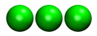
You may need to adjust the van der Waals radius in your visualization program to see the atoms colliding.
10.4. HelloSodiumChloride Program
The HelloSodiumChloride models several sodium (Na+) and chloride (Cl-) ions in implicit solvent (using a Generalized Born/Surface Area, or GBSA, OBC model). As with the HelloArgon program, only non-bonded forces are simulated.
The main purpose of this example is to illustrate our recommended strategy for integrating OpenMM into an existing molecular dynamics (MD) code:
Write a few, high-level interface routines containing all your OpenMM calls: Rather than make OpenMM calls throughout your program, we recommend writing a handful of interface routines that understand both your MD code’s data structures and OpenMM. Organize these routines into a separate compilation unit so you do not have to make huge changes to your existing MD code. These routines could be written in any language that is callable from the existing MD code. We recommend writing them in C++ since that is what OpenMM is written in, but you can also write them in C or Fortran; see Chapter 12.
Call only these high-level interface routines from your existing MD code: This provides a clean separation between the existing MD code and OpenMM, so that changes to OpenMM will not directly impact the existing MD code. One way to implement this is to use opaque handles, a standard trick used (for example) for opening files in Linux. An existing MD code can communicate with OpenMM via the handle, but knows none of the details of the handle. It only has to hold on to the handle and give it back to OpenMM.
In the example described below, you will see how this strategy can be implemented for a very simple MD code. Chapter 13 describes the strategies used in integrating OpenMM into real MD codes.
10.4.1. Simple molecular dynamics system
The initial sections of HelloSodiumChloride.cpp represent a very simple
molecular dynamics system. The system includes modeling and simulation
parameters and the atom and force field data. It also provides a data structure
posInAng[3] for storing the current state. These sections represent
(in highly simplified form) information that would be available from an existing
MD code, and will be used to demonstrate how to integrate OpenMM with an
existing MD program.
// -----------------------------------------------------------------
//                   MODELING AND SIMULATION PARAMETERS
// -----------------------------------------------------------------
static const double Temperature         = 300;     // Kelvins
static const double FrictionInPerPs     = 91.;     // collisions per picosecond
static const double SolventDielectric   = 80.;     // typical for water
static const double SoluteDielectric    = 2.;      // typical for protein

static const double StepSizeInFs        = 4;       // integration step size (fs)
static const double ReportIntervalInFs  = 50;      // how often to issue PDB frame (fs)
static const double SimulationTimeInPs  = 100;     // total simulation time (ps)

// Decide whether to request energy calculations.
static const bool   WantEnergy          = true;


// -----------------------------------------------------------------
//                          ATOM AND FORCE FIELD DATA
// -----------------------------------------------------------------
// This is not part of OpenMM; just a struct we can use to collect atom
// parameters for this example. Normally atom parameters would come from the
// force field's parameterization file. We're going to use data in Angstrom and
// Kilocalorie units and show how to safely convert to OpenMM's internal unit
// system which uses nanometers and kilojoules.
static struct MyAtomInfo {
    const char* pdb;
    double      mass, charge, vdwRadiusInAng, vdwEnergyInKcal,
                gbsaRadiusInAng, gbsaScaleFactor;
    double      initPosInAng[3];
    double      posInAng[3]; // leave room for runtime state info
} atoms[] = {
// pdb   mass  charge  vdwRad vdwEnergy   gbsaRad gbsaScale  initPos
{" NA ", 22.99,  1,    1.8680, 0.00277,    1.992,   0.8,     8, 0,  0},
{" CL ", 35.45, -1,    2.4700, 0.1000,     1.735,   0.8,    -8, 0,  0},
{" NA ", 22.99,  1,    1.8680, 0.00277,    1.992,   0.8,     0, 9,  0},
{" CL ", 35.45, -1,    2.4700, 0.1000,     1.735,   0.8,     0,-9,  0},
{" NA ", 22.99,  1,    1.8680, 0.00277,    1.992,   0.8,     0, 0,-10},
{" CL ", 35.45, -1,    2.4700, 0.1000,     1.735,   0.8,     0, 0, 10},
{""} // end of list
};
10.4.2. Interface routines
The key to our recommended integration strategy is the interface routines. You will need to decide what interface routines are required for effective communication between your existing MD program and OpenMM, but typically there will only be six or seven. In our example, the following four routines suffice:
Initialize: Data structures that already exist in your MD program (i.e., force fields, constraints, atoms in the system) are passed to the
Initializeroutine, which makes appropriate calls to OpenMM and then returns a handle to the OpenMM object that can be used by the existing MD program.Terminate: Clean up the heap space allocated by
Initializeby passing the handle to theTerminateroutine.Advance State: The
AdvanceStateroutine advances the simulation. It requires that the calling function, the existing MD code, gives it a handle.Retrieve State: When you want to do an analysis or generate some kind of report, you call the
RetrieveStateroutine. You have to give it a handle. It then fills in a data structure that is defined in the existing MD code, allowing the MD program to use it in its existing routines without further modification.
Note that these are just descriptions of the routines’ functions—you can call them anything you like and implement them in whatever way makes sense for your MD code.
In the example code, the four routines performing these functions, plus an
opaque data structure (the handle), would be declared, as shown below. Then,
the main program, which sets up, runs, and reports on the simulation, accesses
these routines and the opaque data structure (in this case, the variable
omm). As you can see, it does not have access to any OpenMM
declarations, only to the interface routines that you write so there is no need
to change the build environment.
struct MyOpenMMData;
static MyOpenMMData* myInitializeOpenMM(const MyAtomInfo atoms[],
                                        double temperature,
                                        double frictionInPs,
                                        double solventDielectric,
                                        double soluteDielectric,
                                        double stepSizeInFs,
                                        std::string& platformName);
static void          myStepWithOpenMM(MyOpenMMData*, int numSteps);
static void          myGetOpenMMState(MyOpenMMData*,
                                      bool wantEnergy,
                                      double& time,
                                      double& energy,
                                      MyAtomInfo atoms[]);
static void          myTerminateOpenMM(MyOpenMMData*);


// -----------------------------------------------------------------
//                                MAIN PROGRAM
// -----------------------------------------------------------------
int main() {
    const int NumReports     = (int)(SimulationTimeInPs*1000 / ReportIntervalInFs + 0.5);
    const int NumSilentSteps = (int)(ReportIntervalInFs / StepSizeInFs + 0.5);

    // ALWAYS enclose all OpenMM calls with a try/catch block to make sure that
    // usage and runtime errors are caught and reported.
    try {
        double        time, energy;
        std::string   platformName;

        // Set up OpenMM data structures; returns OpenMM Platform name.
        MyOpenMMData* omm = myInitializeOpenMM(atoms, Temperature, FrictionInPerPs,
             SolventDielectric, SoluteDielectric, StepSizeInFs, platformName);

        // Run the simulation:
        //  (1) Write the first line of the PDB file and the initial configuration.
        //  (2) Run silently entirely within OpenMM between reporting intervals.
        //  (3) Write a PDB frame when the time comes.
        printf("REMARK  Using OpenMM platform %s\n", platformName.c_str());
        myGetOpenMMState(omm, WantEnergy, time, energy, atoms);
        myWritePDBFrame(1, time, energy, atoms);

        for (int frame=2; frame <= NumReports; ++frame) {
            myStepWithOpenMM(omm, NumSilentSteps);
            myGetOpenMMState(omm, WantEnergy, time, energy, atoms);
            myWritePDBFrame(frame, time, energy, atoms);
        }

        // Clean up OpenMM data structures.
        myTerminateOpenMM(omm);

        return 0; // Normal return from main.
    }

    // Catch and report usage and runtime errors detected by OpenMM and fail.
    catch(const std::exception& e) {
        printf("EXCEPTION: %s\n", e.what());
        return 1;
    }
}
We will examine the implementation of each of the four interface routines and the opaque data structure (handle) in the sections below.
Units
The simple molecular dynamics system described in Section 10.4.1 employs the commonly used units of angstroms and kcals. These differ from the units and parameters used within OpenMM (see Section 18.2): nanometers and kilojoules. These differences may be small but they are critical and must be carefully accounted for in the interface routines.
Lennard-Jones potential
The Lennard-Jones potential describes the energy between two identical atoms as the distance between them varies.
The van der Waals “size” parameter is used to identify the distance at which the energy between these two atoms is at a minimum (that is, where the van der Waals force is most attractive). There are several ways to specify this parameter, typically, either as the van der Waals radius rvdw or as the actual distance between the two atoms dmin (also called rmin), which is twice the van der Waals radius rvdw. A third way to describe the potential is through sigma \(\sigma\), which identifies the distance at which the energy function crosses zero as the atoms move closer together than dmin. (See Section 19.6.1 for more details about the relationship between these).
\(\sigma\) turns out to be about 0.89*dmin, which is close enough to dmin that it makes it hard to distinguish the two. Be very careful that you use the correct value. In the example below, we will show you how to use the built-in OpenMM conversion constants to avoid errors.
Lennard-Jones parameters are defined for pairs of identical atoms, but must also be applied to pairs of dissimilar atoms. That is done by “combining rules” that differ among popular MD codes. Two of the most common are:
Lorentz-Berthelot (used by AMBER, CHARMM):
Jorgensen (used by OPLS):
where r = the effective van der Waals “size” parameter (minimum radius, minimum distance, or zero crossing (sigma)), and \(\epsilon\) = the effective van der Waals energy well depth parameter, for the dissimilar pair of atoms i and j.
OpenMM only implements Lorentz-Berthelot directly, but others can be implemented using the CustomNonbondedForce class. (See Section 20.4 for details.)
Opaque handle MyOpenMMData
In this example, the handle used by the interface to OpenMM is a pointer to a
struct called MyOpenMMData. The pointer itself is opaque, meaning
the calling program has no knowledge of what the layout of the object it points
to is, or how to use it to directly interface with OpenMM. The calling program
will simply pass this opaque handle from one interface routine to another.
There are many different ways to implement the handle. The code below shows just one example. A simulation requires three OpenMM objects (a System, a Context, and an Integrator) and so these must exist within the handle. If other objects were required for a simulation, you would just add them to your handle; there would be no change in the main program using the handle.
struct MyOpenMMData {
    MyOpenMMData() : system(0), context(0), integrator(0) {}
    ~MyOpenMMData() {delete system; delete context; delete integrator;}
    OpenMM::System*         system;
    OpenMM::Context*        context;
    OpenMM::Integrator*     integrator;
};
In addition to establishing pointers to the required three OpenMM objects,
MyOpenMMData has a constructor MyOpenMMData() that sets
the pointers for the three OpenMM objects to zero and a destructor
~MyOpenMMData() that (in C++) gives the heap space back. This was
done in-line in the HelloArgon program, but we recommend you use something like
the method here instead.
myInitializeOpenMM
The myInitializeOpenMM function takes the data structures and
simulation parameters from the existing MD code and returns a new handle that
can be used to do efficient computations with OpenMM. It also returns the
platformName so the calling program knows what platform (e.g., CUDA,
OpenCL, Reference) was used.
static MyOpenMMData*
myInitializeOpenMM( const MyAtomInfo    atoms[],
                    double              temperature,
                    double              frictionInPs,
                    double              solventDielectric,
                    double              soluteDielectric,
                    double              stepSizeInFs,
                    std::string&        platformName)
This initialization routine is very similar to the HelloArgon example program,
except that objects are created and put in the handle. For instance, just as in
the HelloArgon program, the first step is to load the OpenMM plug-ins, so that
the program will run on the best performing platform that is available. Then,
a System is created and assigned to the handle omm.
Similarly, forces are added to the System which is already in the handle.
// Load all available OpenMM plugins from their default location.
OpenMM::Platform::loadPluginsFromDirectory
       (OpenMM::Platform::getDefaultPluginsDirectory());

// Allocate space to hold OpenMM objects while we're using them.
MyOpenMMData* omm = new MyOpenMMData();

// Create a System and Force objects within the System. Retain a reference
// to each force object so we can fill in the forces. Note: the OpenMM
// System takes ownership of the force objects;don't delete them yourself.
omm->system = new OpenMM::System();
OpenMM::NonbondedForce* nonbond = new OpenMM::NonbondedForce();
OpenMM::GBSAOBCForce*   gbsa    = new OpenMM::GBSAOBCForce();
omm->system->addForce(nonbond);
omm->system->addForce(gbsa);

// Specify dielectrics for GBSA implicit solvation.
gbsa->setSolventDielectric(solventDielectric);
gbsa->setSoluteDielectric(soluteDielectric);
In the next step, atoms are added to the System within the handle, with
information about each atom coming from the data structure that was passed into
the initialization function from the existing MD code. As shown in the
HelloArgon program, both the System and the forces need information about the
atoms. For those unfamiliar with the C++ Standard Template Library, the
push_back function called at the end of this code snippet just adds
the given argument to the end of a C++ “vector” container.
// Specify the atoms and their properties:
//  (1) System needs to know the masses.
//  (2) NonbondedForce needs charges,van der Waals properties(in MD units!).
//  (3) GBSA needs charge, radius, and scale factor.
//  (4) Collect default positions for initializing the simulation later.
std::vector<Vec3> initialPosInNm;
for (int n=0; *atoms[n].pdb; ++n) {
     const MyAtomInfo& atom = atoms[n];

     omm->system->addParticle(atom.mass);

     nonbond->addParticle(atom.charge,
                         atom.vdwRadiusInAng * OpenMM::NmPerAngstrom
                                             * OpenMM::SigmaPerVdwRadius,
                         atom.vdwEnergyInKcal * OpenMM::KJPerKcal);

     gbsa->addParticle(atom.charge,
                       atom.gbsaRadiusInAng * OpenMM::NmPerAngstrom,
                       atom.gbsaScaleFactor);

     // Convert the initial position to nm and append to the array.
     const Vec3 posInNm(atom.initPosInAng[0] * OpenMM::NmPerAngstrom,
                  atom.initPosInAng[1] * OpenMM::NmPerAngstrom,
                  atom.initPosInAng[2] * OpenMM::NmPerAngstrom);
     initialPosInNm.push_back(posInNm);
Units: Here we emphasize the need to pay special attention to the units. As mentioned earlier, the existing MD code in this example uses units of angstroms and kcals, but OpenMM uses nanometers and kilojoules. So the initialization routine will need to convert the values from the existing MD code into the OpenMM units before assigning them to the OpenMM objects.
In the code above, we have used the unit conversion constants that come with
OpenMM (e.g., OpenMM::NmPerAngstrom) to perform these conversions.
Combined with the naming convention of including the units in the variable name
(e.g., initPosInAng), the unit conversion constants are useful
reminders to pay attention to units and minimize errors.
Finally, the initialization routine creates the Integrator and Context for the
simulation. Again, note the change in units for the arguments! The routine
then gets the platform that will be used to run the simulation and returns that,
along with the handle omm, back to the calling function.
// Choose an Integrator for advancing time, and a Context connecting the
// System with the Integrator for simulation. Let the Context choose the
// best available Platform. Initialize the configuration from the default
// positions we collected above. Initial velocities will be zero but could
// have been set here.
omm->integrator = new OpenMM::LangevinMiddleIntegrator(temperature,
frictionInPs,
stepSizeInFs * OpenMM::PsPerFs);
omm->context    = new OpenMM::Context(*omm->system, *omm->integrator);
omm->context->setPositions(initialPosInNm);

platformName = omm->context->getPlatform().getName();
return omm;
myGetOpenMMState
The myGetOpenMMState function takes the handle and returns the time,
energy, and data structure for the atoms in a way that the existing MD code can
use them without modification.
static void
myGetOpenMMState(MyOpenMMData* omm, bool wantEnergy,
                 double& timeInPs, double& energyInKcal, MyAtomInfo atoms[])
Again, this is another interface routine in which you need to be very careful of your units! Note the conversion from the OpenMM units back to the units used in the existing MD code.
int infoMask = 0;
infoMask = OpenMM::State::Positions;
if (wantEnergy) {
   infoMask += OpenMM::State::Velocities; // for kinetic energy (cheap)
   infoMask += OpenMM::State::Energy;     // for pot. energy (more expensive)
}
// Forces are also available (and cheap).

const OpenMM::State state = omm->context->getState(infoMask);
timeInPs = state.getTime(); // OpenMM time is in ps already

// Copy OpenMM positions into atoms array and change units from nm to Angstroms.
const std::vector<Vec3>& positionsInNm = state.getPositions();
for (int i=0; i < (int)positionsInNm.size(); ++i)
    for (int j=0; j < 3; ++j)
         atoms[i].posInAng[j] = positionsInNm[i][j] * OpenMM::AngstromsPerNm;

// If energy has been requested, obtain it and convert from kJ to kcal.
energyInKcal = 0;
if (wantEnergy)
   energyInKcal = (state.getPotentialEnergy() + state.getKineticEnergy())
                  * OpenMM::KcalPerKJ;
myStepWithOpenMM
The myStepWithOpenMM routine takes the handle, uses it to find the
Integrator, and then sets the number of steps for the Integrator to take. It
does not return any values.
static void
myStepWithOpenMM(MyOpenMMData* omm, int numSteps) {
    omm->integrator->step(numSteps);
}
myTerminateOpenMM
The myTerminateOpenMM routine takes the handle and deletes all the
components, e.g., the Context and System, cleaning up the heap space.
static void
myTerminateOpenMM(MyOpenMMData* omm) {
    delete omm;
}
10.5. HelloEthane Program
The HelloEthane program simulates ethane (H3-C-C-H3) in a vacuum. It is structured similarly to the HelloSodiumChloride example, but includes bonded forces (bond stretch, bond angle bend, dihedral torsion). In setting up these bonded forces, the program illustrates some of the other inconsistencies in definitions and units that you should watch out for.
The bonded forces are added to the system within the initialization interface routine, similar to how the non-bonded forces were added in the HelloSodiumChloride example:
// Create a System and Force objects within the System. Retain a reference
// to each force object so we can fill in the forces. Note: the System owns
// the force objects and will take care of deleting them; don't do it yourself!
OpenMM::System&                 system      = *(omm->system = new OpenMM::System());
OpenMM::NonbondedForce&         nonbond     = *new OpenMM::NonbondedForce();
OpenMM::HarmonicBondForce&      bondStretch = *new OpenMM::HarmonicBondForce();
OpenMM::HarmonicAngleForce&     bondBend    = *new OpenMM::HarmonicAngleForce();
OpenMM::PeriodicTorsionForce&   bondTorsion = *new OpenMM::PeriodicTorsionForce();
system.addForce(&nonbond);
system.addForce(&bondStretch);
system.addForce(&bondBend);
system.addForce(&bondTorsion);
Constrainable and non-constrainable bonds: In the initialization routine, we also set up the bonds. If constraints are being used, then we tell the System about the constrainable bonds:
std::vector< std::pair<int,int> > bondPairs;
for (int i=0; bonds[i].type != EndOfList; ++i) {
    const int*      atom = bonds[i].atoms;
    const BondType& bond = bondType[bonds[i].type];

    if (UseConstraints && bond.canConstrain) {
        system.addConstraint(atom[0], atom[1],
                bond.nominalLengthInAngstroms * OpenMM::NmPerAngstrom);
    }
Otherwise, we need to give the HarmonicBondForce the bond stretch parameters.
Warning: The constant used to specify the stiffness may be defined differently between the existing MD code and OpenMM. For instance, AMBER uses the constant, as given in the harmonic energy term kx2, where the force is 2kx (k = constant and x = distance). OpenMM wants the constant, as used in the force term kx (with energy 0.5 * kx2). So a factor of 2 must be introduced when setting the bond stretch parameters in an OpenMM system using data from an AMBER system.
bondStretch.addBond(atom[0], atom[1], bond.nominalLengthInAngstroms * OpenMM::NmPerAngstrom,
                    bond.stiffnessInKcalPerAngstrom2 * 2 * OpenMM::KJPerKcal *
                    OpenMM::AngstromsPerNm * OpenMM::AngstromsPerNm);
Non-bond exclusions: Next, we deal with non-bond exclusions. These are used for pairs of atoms that appear close to one another in the network of bonds in a molecule. For atoms that close, normal non-bonded forces do not apply or are reduced in magnitude. First, we create a list of bonds to generate the non- bond exclusions:
bondPairs.push_back(std::make_pair(atom[0], atom[1]));
OpenMM’s non-bonded force provides a convenient routine for creating the common exceptions. These are: (1) for atoms connected by one bond (1-2) or connected by just one additional bond (1-3), Coulomb and van der Waals terms do not apply; and (2) for atoms connected by three bonds (1-4), Coulomb and van der Waals terms apply but are reduced by a force-field dependent scale factor. In general, you may introduce additional exceptions, but the standard ones suffice here and in many other circumstances.
// Exclude 1-2, 1-3 bonded atoms from nonbonded forces, and scale down 1-4 bonded atoms.
nonbond.createExceptionsFromBonds(bondPairs, Coulomb14Scale, LennardJones14Scale);

// Create the 1-2-3 bond angle harmonic terms.
for (int i=0; angles[i].type != EndOfList; ++i) {
     const int*       atom  = angles[i].atoms;
     const AngleType& angle = angleType[angles[i].type];

// See note under bond stretch above regarding the factor of 2 here.
bondBend.addAngle(atom[0],atom[1],atom[2],
angle.nominalAngleInDegrees     * OpenMM::RadiansPerDegree,
angle.stiffnessInKcalPerRadian2 * 2 *
OpenMM::KJPerKcal);
}

// Create the 1-2-3-4 bond torsion (dihedral) terms.
for (int i=0; torsions[i].type != EndOfList; ++i) {
     const int*         atom = torsions[i].atoms;
    const TorsionType& torsion = torsionType[torsions[i].type];
    bondTorsion.addTorsion(atom[0],atom[1],atom[2],atom[3],
            torsion.periodicity,
            torsion.phaseInDegrees  * OpenMM::RadiansPerDegree,
            torsion.amplitudeInKcal * OpenMM::KJPerKcal);
}
The rest of the code is similar to the HelloSodiumChloride example and will not be covered in detail here. Please refer to the program HelloEthane.cpp itself, which is well-commented, for additional details.