14. Testing and Validation of OpenMM
The goal of testing and validation is to make sure that OpenMM works correctly. That means that it runs without crashing or otherwise failing, and that it produces correct results. Furthermore, it must work correctly on a variety of hardware platforms (e.g. different models of GPU), software platforms (e.g. operating systems and OpenCL implementations), and types of simulations.
Three types of tests are used to validate OpenMM:
Unit tests: These are small tests designed to test specific features or pieces of code in isolation. For example, a test of HarmonicBondForce might create a System with just a few particles and bonds, compute the forces and energy, and compare them to the analytically expected values. There are thousands of unit tests that collectively cover all of OpenMM.
System tests: Whereas unit tests validate small features in isolation, system tests are designed to validate the entire library as a whole. They simulate realistic models of biomolecules and perform tests that are likely to fail if any problem exists anywhere in the library.
Direct comparison between OpenMM and other programs: The third type of validation performed is a direct comparison of the individual forces computed by OpenMM to those computed by other programs for a collection of biomolecules.
Each type of test is outlined in greater detail below; a discussion of the current status of the tests is then given.
14.1. Description of Tests
14.1.1. Unit tests
The unit tests are with the source code, so if you build from source you can run them yourself. See Section 9.1.4 for details. When you run the tests (for example, by typing “make test” on Linux or Mac), it should produce output something like this:
      Start   1: TestReferenceAndersenThermostat
1/317 Test   #1: TestReferenceAndersenThermostat .............. Passed  0.26 sec
      Start   2: TestReferenceBrownianIntegrator
2/317 Test   #2: TestReferenceBrownianIntegrator .............. Passed  0.13 sec
      Start   3: TestReferenceCheckpoints
3/317 Test   #3: TestReferenceCheckpoints ..................... Passed  0.02 sec
... <many other tests> ...
Each line represents a test suite, which may contain multiple unit tests. If all tests within a suite passed, it prints the word “Passed” and how long the suite took to execute. Otherwise it prints an error message. If any tests failed, you can then run them individually (each one is a separate executable) to get more details on what went wrong.
14.1.2. System tests
Several different types of system tests are performed. Each type is run for a variety of systems, including both proteins and nucleic acids, and involving both implicit and explicit solvent. The full suite of tests is repeated for both the CUDA and OpenCL platforms, using both single and double precision (and for the integration tests, mixed precision as well), on a variety of operating systems and hardware. There are four types of tests:
Consistency between platforms: The forces and energy are computed using the platform being tested, then compared to ones computed with the Reference platform. The results are required to agree to within a small tolerance.
Energy-force consistency: This verifies that the force really is the gradient of the energy. It first computes the vector of forces for a given conformation. It then generates four other conformations by displacing the particle positions by small amounts along the force direction. It computes the energy of each one, uses those to calculate a fourth order finite difference approximation to the derivative along that direction, and compares it to the actual forces. They are required to agree to within a small tolerance.
Energy conservation: The system is simulated at constant energy using a Verlet integrator, and the total energy is periodically recorded. A linear regression is used to estimate the rate of energy drift. In addition, all constrained distances are monitored during the simulation to make sure they never differ from the expected values by more than the constraint tolerance.
Thermostability: The system is simulated at constant temperature using a Langevin integrator. The mean kinetic energy over the course of the simulation is computed and compared to the expected value based on the temperature. In addition, all constrained distances are monitored during the simulation to make sure they never differ from the expected values by more than the constraint tolerance.
If you want to run the system tests yourself, they can be found in the Subversion repository at https://simtk.org/svn/pyopenmm/trunk/test/system-tests. Check out that directory, then execute the runAllTests.sh shell script. It will create a series of files with detailed information about the results of the tests. Be aware that running the full test suite may take a long time (possibly several days) depending on the speed of your GPU.
14.1.3. Direct comparisons between OpenMM and other programs
As a final check, identical systems are set up in OpenMM and in another program (Gromacs 4.5 or Tinker 6.1), each one is used to compute the forces on atoms, and the results are directly compared to each other.
14.2. Test Results
In this section, we highlight the major results obtained from the tests described above. They are not exhaustive, but should give a reasonable idea of the level of accuracy you can expect from OpenMM.
14.2.1. Comparison to Reference Platform
The differences between forces computed with the Reference platform and those computed with the OpenCL or CUDA platform are shown in Table 14-1. For every atom, the relative difference between platforms was computed as 2·|Fref–Ftest|/(|Fref|+|Ftest|), where Fref is the force computed by the Reference platform and Ftest is the force computed by the platform being tested (OpenCL or CUDA). The median over all atoms in a given system was computed to estimate the typical force errors for that system. Finally, the median of those values for all test systems was computed to give the value shown in the table.
Force |
OpenCL (single) |
OpenCL (double) |
CUDA (single) |
CUDA (double) |
|---|---|---|---|---|
Total Force |
2.53·10-6 |
1.44·10-7 |
2.56·10-6 |
8.78·10-8 |
HarmonicBondForce |
2.88·10-6 |
1.57·10-13 |
2.88·10-6 |
1.57·10-13 |
HarmonicAngleForce |
2.25·10-5 |
4.21·10-7 |
2.27·10-5 |
4.21·10-7 |
PeriodicTorsionForce |
8.23·10-7 |
2.44·10-7 |
9.27·10-7 |
2.56·10-7 |
RBTorsionForce |
4.86·10-6 |
1.46·10-7 |
4.72·10-6 |
1.4·10-8 |
NonbondedForce (no cutoff) |
1.49·10-6 |
6.49·10-8 |
1.49·10-6 |
6.49·10-8 |
NonbondedForce (cutoff, nonperiodic) |
9.74·10-7 |
4.88·10-9 |
9.73·10-7 |
4.88·10-9 |
NonbondedForce (cutoff, periodic) |
9.82·10-7 |
4.88·10-9 |
9.8·10-7 |
4.88·10-9 |
NonbondedForce (Ewald) |
1.33·10-6 |
5.22·10-9 |
1.33·10-6 |
5.22·10-9 |
NonbondedForce (PME) |
3.99·10-5 |
4.08·10-6 |
3.99·10-5 |
4.08·10-6 |
GBSAOBCForce (no cutoff) |
3.0·10-6 |
1.76·10-7 |
3.09·10-6 |
9.4·10-8 |
GBSAOBCForce (cutoff, nonperiodic) |
2.77·10-6 |
1.76·10-7 |
2.95·10-6 |
9.33·10-8 |
GBSAOBCForce (cutoff, periodic) |
2.61·10-6 |
1.78·10-7 |
2.77·10-6 |
9.24·10-8 |
Table 14-1: Median relative difference in forces between Reference platform and OpenCL/CUDA platform
14.2.2. Energy Conservation
Figure 14-1 shows the total system energy versus time for three simulations of ubiquitin in OBC implicit solvent. All three simulations used the CUDA platform, a Verlet integrator, a time step of 0.5 fs, no constraints, and no cutoff on the nonbonded interactions. They differ only in the level of numeric precision that was used for calculations (see Chapter 11).
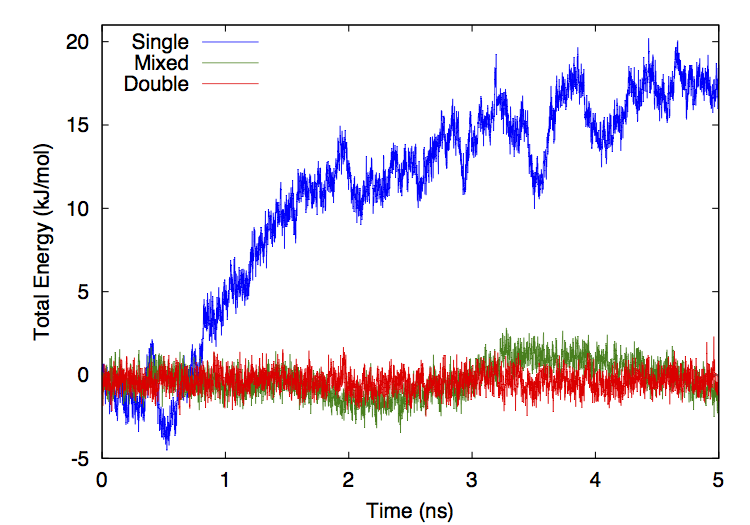
Figure 14-1: Total energy versus time for simulations run in three different precision modes.
For the mixed and double precision simulations, the drift in energy is almost entirely diffusive with negligible systematic drift. The single precision simulation has a more significant upward drift with time, though the rate of drift is still small compared to the rate of short term fluctuations. Fitting a straight line to each curve gives a long term rate of energy drift of 3.98 kJ/mole/ns for single precision, 0.217 kJ/mole/ns for mixed precision, and 0.00100 kJ/mole/ns for double precision. In the more commonly reported units of kT/ns/dof, these correspond to 4.3·10-4 for single precision, 2.3·10-5 for mixed precision, and 1.1·10-7 for double precision.
Be aware that different simulation parameters will give different results. These simulations were designed to minimize all sources of error except those inherent in OpenMM. There are other sources of error that may be significant in other situations. In particular:
Using a larger time step increases the integration error (roughly proportional to dt2).
If a system involves constraints, the level of error will depend strongly on the constraint tolerance specified by the Integrator.
When using Ewald summation or Particle Mesh Ewald, the accuracy will depend strongly on the Ewald error tolerance.
Applying a distance cutoff to implicit solvent calculations will increase the error, and the shorter the cutoff is, the greater the error will be.
As a result, the rate of energy drift may be much greater in some simulations than in the ones shown above.
14.2.3. Comparison to Gromacs
OpenMM and Gromacs 4.5.5 were each used to compute the atomic forces for
dihydrofolate reductase (DHFR) in implicit and explicit solvent. The implicit
solvent calculations used the OBC solvent model and no cutoff on nonbonded
interactions. The explicit solvent calculations used Particle Mesh Ewald and a
1 nm cutoff on direct space interactions. For OpenMM, the Ewald error tolerance
was set to 10-6. For Gromacs, fourierspacing was set to
0.07 and ewald_rtol to 10-6. No constraints were applied
to any degrees of freedom. Both programs used single precision. The test was
repeated for OpenCL, CUDA, and CPU platforms.
For every atom, the relative difference between OpenMM and Gromacs was computed as 2·|FMM–FGro|/(|FMM|+|FGro|), where FMM is the force computed by OpenMM and FGro is the force computed by Gromacs. The median over all atoms is shown in Table 14-2.
Solvent Model |
OpenCL |
CUDA |
CPU |
|---|---|---|---|
Implicit |
7.66·10-6 |
7.68·10-6 |
1.94·10-5 |
Explicit |
6.77·10-5 |
6.78·10-5 |
9.89·10-5 |
Table 14-2: Median relative difference in forces between OpenMM and Gromacs